library(tidyverse)library(sf)library(spdep)library(spatstat)library(mapview)
library(viridis)library(knitr)
library(patchwork)library(tidyverse)library(sf)library(spdep)library(spatstat)library(mapview)
library(viridis)library(knitr)
library(patchwork)The systematic destruction of Black communities through urban interventions has left lasting imprints on American cities. During the mid-twentieth century, the Home Owners’ Loan Corporation (HOLC) created “residential security maps” that classified neighborhoods by perceived investment risk. Areas with significant Black populations were systematically marked as “hazardous” (Grade D, colored red on maps)—a practice that became known as “redlining.”
Brooklyn’s East New York neighborhood exemplifies this pattern. Once a thriving community, East New York was heavily redlined in the 1930s, setting in motion decades of disinvestment and spatial inequality. This study investigates whether these historical interventions continue to shape contemporary patterns of racial composition and income in Brooklyn.
Do the 1930s HOLC redlining zones in Brooklyn continue to shape the spatial distribution of race and income in these areas today?
I hypothesize that:
HOLC Redlining Maps (1930s)
Historical “residential security” maps from the Mapping Inequality project, showing Grade A (green/best), B (blue), C (yellow), and D (red/hazardous) zones in Brooklyn.
Census Data (1990-2020)
Time series demographic and income data from the National Historical Geographic Information System (NHGIS):
My analysis focuses on Brooklyn (Kings County), New York, with particular attention to East New York—an area in eastern Brooklyn with high concentrations of D-grade (redlined) zones. I identified 161 census tracts in eastern Brooklyn where >25% of the tract area overlaps with redlined zones.
First, let’s load the processed data and examine the basic patterns.
# Load processed data
redline <- st_read("data/raw/brooklyn.json", quiet = TRUE)
tracts_2020 <- st_read("data/processed/brooklyn_tracts_with_data_2020.gpkg",
                       quiet = TRUE)
east_ny_tracts <- read_csv("data/processed/east_new_york_tracts.csv",
                           show_col_types = FALSE)

# Calculate demographic variables for 2020
tracts_2020 <- tracts_2020 %>%
  mutate(
    # Total population
    total_pop = CV4AA2020 + CV4AB2020 + CV4AC2020 + CV4AD2020 + CV4AE2020 +
                CV4AF2020 + CV4AG2020 + CV4AH2020 + CV4AI2020 + CV4AJ2020,
    # Total Black population (Non-Hispanic + Hispanic)
    black_total = CV4AB2020 + CV4AG2020,
    # Percent Black (including Afro-Latinos)
    pct_black = ifelse(total_pop > 0, (black_total / total_pop) * 100, NA),
    # Median household income (2018-2022)
    med_income = B79AA225,
    # Flag East New York tracts
    is_east_ny = GISJOIN %in% east_ny_tracts$GISJOIN
)# Overall summary
cat("Brooklyn Census Tracts (2020):", nrow(tracts_2020), "\n")Brooklyn Census Tracts (2020): 804 cat("East New York Tracts:", sum(tracts_2020$is_east_ny), "\n\n")East New York Tracts: 161 # Summary by East New York status
summary_table <- tracts_2020 %>%
st_drop_geometry() %>%
group_by(is_east_ny) %>%
summarize(
n_tracts = n(),
mean_pct_black = mean(pct_black, na.rm = TRUE),
median_income = median(med_income, na.rm = TRUE),
.groups = "drop"
) %>%
mutate(area = ifelse(is_east_ny, "East New York (Redlined)",
"Rest of Brooklyn"))
kable(summary_table %>% select(area, n_tracts, mean_pct_black, median_income),
col.names = c("Area", "N Tracts", "Mean % Black", "Median Income"),
digits = 2)| Area | N Tracts | Mean % Black | Median Income |
|---|---|---|---|
| Rest of Brooklyn | 643 | 3.92 | 76908 |
| East New York (Redlined) | 161 | 9.12 | 69365 |
ggplot() +
  geom_sf(data = tracts_2020, aes(fill = pct_black), color = NA) +
  scale_fill_viridis_c(option = "plasma", na.value = "grey90",
                       name = "% Black\n(2020)",
                       labels = scales::percent_format(scale = 1)) +
  geom_sf(data = redline, aes(color = grade), fill = NA, linewidth = 0.8) +
  scale_color_manual(values = c("A" = "#76a865", "B" = "#7cb5bd",
                                 "C" = "#ffff00", "D" = "#d9838d"),
                     name = "HOLC Grade\n(1930s)") +
  theme_minimal() +
  labs(title = "Black Population Distribution and Historical Redlining",
       subtitle = "Brooklyn, NY (includes Afro-Latinos)")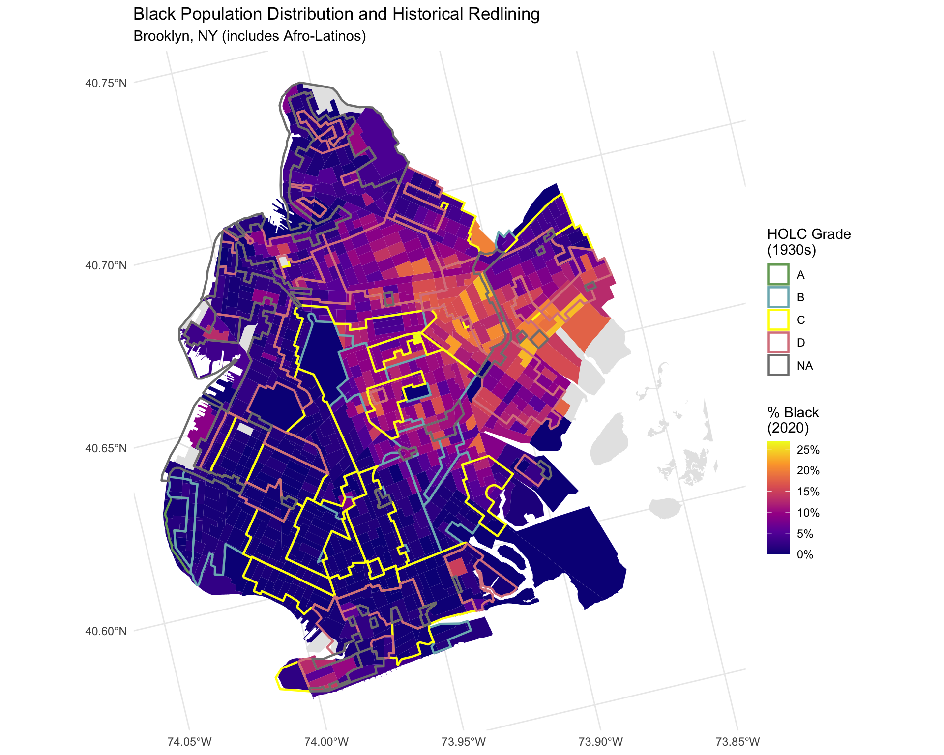
ggplot() +
  geom_sf(data = tracts_2020, aes(fill = med_income), color = NA) +
  scale_fill_viridis_c(option = "mako", na.value = "grey90",
                       name = "Median HH\nIncome ($)",
                       labels = scales::dollar_format()) +
  geom_sf(data = redline, aes(color = grade), fill = NA, linewidth = 0.8) +
  scale_color_manual(values = c("A" = "#76a865", "B" = "#7cb5bd",
                                 "C" = "#ffff00", "D" = "#d9838d"),
                     name = "HOLC Grade\n(1930s)") +
  theme_minimal() +
  labs(title = "Median Household Income and Historical Redlining",
       subtitle = "Brooklyn, NY")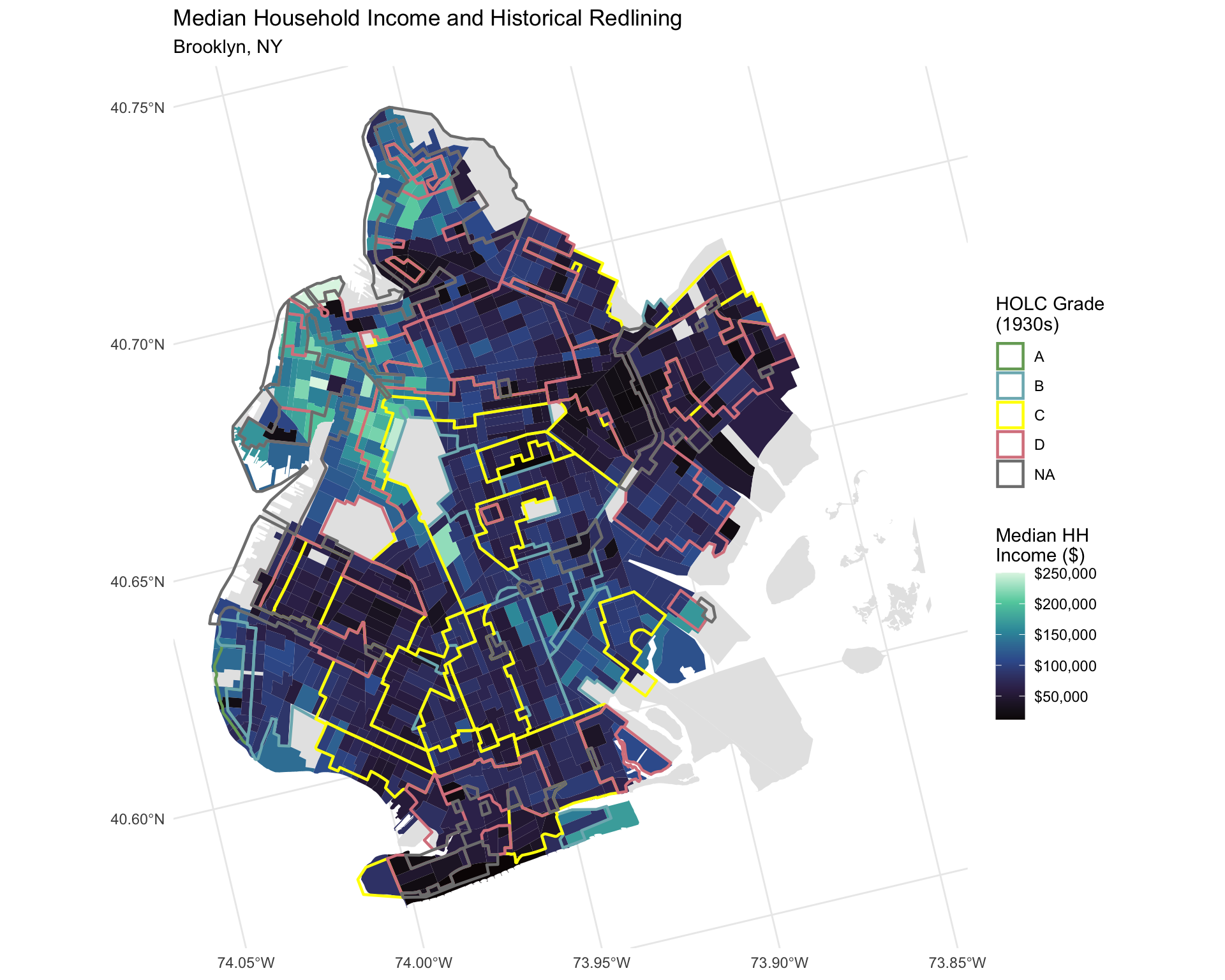
We now test for global spatial autocorrelation using Moran’s I. This measures whether similar values cluster together more than would be expected by chance.
# Create spatial weights matrix (Queen contiguity)
# Remove tracts with missing values
tracts_complete <- tracts_2020 %>%
  filter(!is.na(pct_black), !is.na(med_income))

# Create neighbors
nb <- poly2nb(tracts_complete, queen = TRUE)
# Create spatial weights
lw <- nb2listw(nb, style = "W", zero.policy = TRUE)

# Moran's I for percent Black
moran_black <- moran.test(tracts_complete$pct_black, lw, zero.policy = TRUE)
cat("Moran's I for % Black Population:\n")
Moran's I for % Black Population:cat(sprintf(" I = %.4f\n", moran_black$estimate["Moran I statistic"])) I = 0.7711cat(sprintf(" p-value = %.4e\n", moran_black$p.value)) p-value = 7.6314e-293cat(sprintf(" Interpretation: %s\n\n",
ifelse(moran_black$p.value < 0.05,
"Significant spatial clustering detected",
"No significant clustering"))) Interpretation: Significant spatial clustering detected# Moran's I for income
moran_income <- moran.test(tracts_complete$med_income, lw,
zero.policy = TRUE)
cat("Moran's I for Median Household Income:\n")Moran's I for Median Household Income:cat(sprintf(" I = %.4f\n", moran_income$estimate["Moran I statistic"])) I = 0.5915cat(sprintf(" p-value = %.4e\n", moran_income$p.value)) p-value = 7.5822e-174cat(sprintf(" Interpretation: %s\n",
ifelse(moran_income$p.value < 0.05,
"Significant spatial clustering detected",
"No significant clustering"))) Interpretation: Significant spatial clustering detectedLISA analysis identifies specific areas of clustering—“hot spots” (high values near high values) and “cold spots” (low values near low values).
# Local Moran's I for percent Black
lisa_black <- localmoran(tracts_complete$pct_black, lw, zero.policy = TRUE)

# Add LISA results to data
tracts_complete <- tracts_complete %>%
  mutate(
    lisa_black_i = lisa_black[, "Ii"],
    lisa_black_p = lisa_black[, "Pr(z != E(Ii))"],
    lisa_black_sig = ifelse(lisa_black_p < 0.05, "Significant", "Not Significant")
  )

# Count significant clusters
cat(sprintf("Significant LISA clusters (p < 0.05): %d out of %d tracts\n",
            sum(tracts_complete$lisa_black_sig == "Significant"),
            nrow(tracts_complete)))
Significant LISA clusters (p < 0.05): 337 out of 772 tractsggplot() +
geom_sf(data = tracts_complete,
aes(fill = lisa_black_i, alpha = lisa_black_sig),
color = "grey40", linewidth = 0.1) +
scale_fill_gradient2(low = "blue", mid = "white", high = "red",
midpoint = 0,
name = "Local\nMoran's I") +
scale_alpha_manual(values = c("Significant" = 1, "Not Significant" = 0.3),
guide = 'none') +
geom_sf(data = redline %>% filter(grade == "D"),
fill = NA, color = "black", linewidth = 0.3, linetype = "solid") +
theme_minimal() +
labs(title = "Local Spatial Autocorrelation (LISA) - Black Population",
subtitle = "Brooklyn, NY (Solid lines = D-grade/redlined zones)")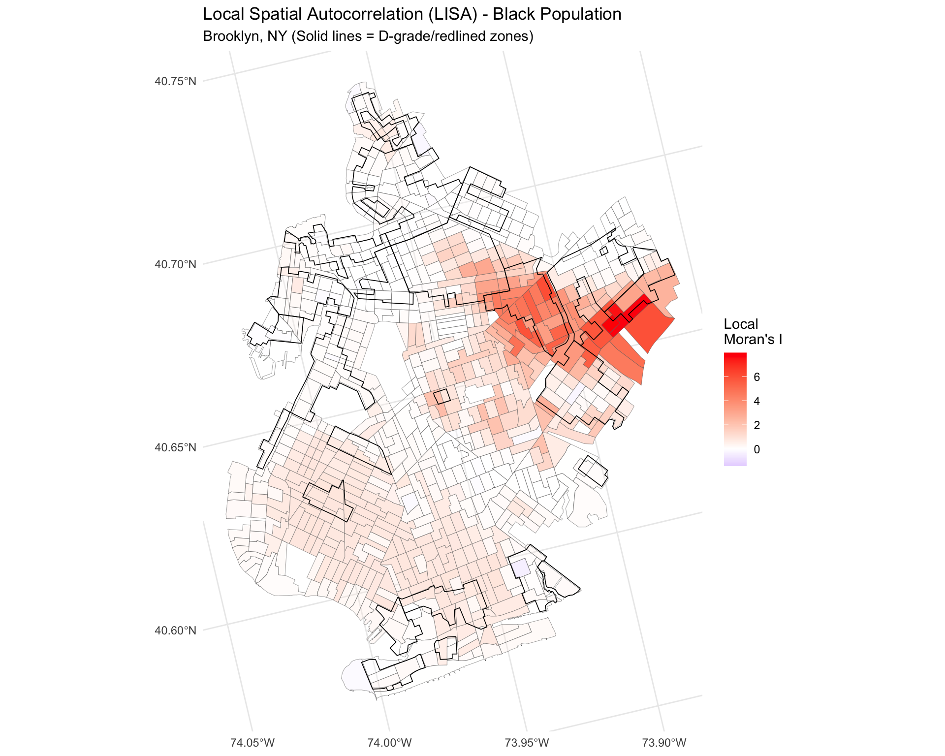
To formally test the hypothesis, I conduct Monte Carlo simulations comparing observed patterns to random spatial distributions.
# Run Monte Carlo simulation for Moran's I (999 permutations)
set.seed(6750)
mc_black <- moran.mc(tracts_complete$pct_black, lw,
                     nsim = 999, zero.policy = TRUE)

cat("Monte Carlo Simulation Results (999 permutations):\n")
Monte Carlo Simulation Results (999 permutations):cat(sprintf(" Observed Moran's I: %.4f\n", mc_black$statistic)) Observed Moran's I: 0.7711cat(sprintf(" p-value: %.4f\n", mc_black$p.value)) p-value: 0.0010cat(sprintf(" Rank: %d out of 1000\n", mc_black$parameter)) Rank: 1000 out of 1000# Plot simulation distribution
hist(mc_black$res,
main = "Monte Carlo Distribution of Moran's I",
xlab = "Moran's I",
col = "lightblue",
breaks = 30)
abline(v = mc_black$statistic, col = "red", lwd = 2)
legend("topright", legend = "Observed Value", col = "red", lwd = 2)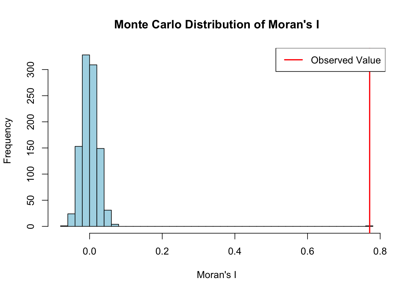
To understand whether redlining’s spatial effects have persisted or changed over time, I compare the spatial autocorrelation patterns between 1990 (60 years after redlining) and 2020 (90 years after redlining).
# Load 1990 data
tracts_1990 <- st_read("data/processed/brooklyn_tracts_with_data_1990.gpkg",
                       quiet = TRUE)

# Calculate demographic variables for 1990
tracts_1990 <- tracts_1990 %>%
  mutate(
    # Total population
    total_pop = CV4AA1990 + CV4AB1990 + CV4AC1990 + CV4AD1990 +
                CV4AF1990 + CV4AG1990 + CV4AH1990 + CV4AI1990,
    # Total Black population (Non-Hispanic + Hispanic)
    black_total = CV4AB1990 + CV4AG1990,
    # Percent Black (including Afro-Latinos)
    pct_black = ifelse(total_pop > 0, (black_total / total_pop) * 100, NA),
    # Median household income (1990)
    med_income = B79AA1990,
    # Flag East New York tracts
    is_east_ny = GISJOIN %in% east_ny_tracts$GISJOIN
  )

# Remove tracts with missing values
tracts_1990_complete <- tracts_1990 %>%
  filter(!is.na(pct_black), !is.na(med_income))

# Create spatial weights for 1990
nb_1990 <- poly2nb(tracts_1990_complete, queen = TRUE)
lw_1990 <- nb2listw(nb_1990, style = "W", zero.policy = TRUE)
# Moran's I for 1990
moran_black_1990 <- moran.test(tracts_1990_complete$pct_black, lw_1990,
zero.policy = TRUE)
# Compare 1990 vs 2020
cat("Temporal Comparison: Spatial Clustering of Black Population\n\n")Temporal Comparison: Spatial Clustering of Black Populationcat(sprintf("1990 (60 years post-redlining):\n"))1990 (60 years post-redlining):cat(sprintf(" Moran's I = %.4f\n", moran_black_1990$estimate["Moran I statistic"])) Moran's I = 0.9154cat(sprintf(" p-value = %.4e\n\n", moran_black_1990$p.value)) p-value = 5.8455e-301cat(sprintf("2020 (90 years post-redlining):\n"))2020 (90 years post-redlining):cat(sprintf(" Moran's I = %.4f\n", moran_black$estimate["Moran I statistic"])) Moran's I = 0.7711cat(sprintf(" p-value = %.4e\n\n", moran_black$p.value)) p-value = 7.6314e-293cat(sprintf("Change over 30 years:\n"))Change over 30 years:i_change <- moran_black$estimate["Moran I statistic"] -
moran_black_1990$estimate["Moran I statistic"]
cat(sprintf(" Δ Moran's I = %.4f\n", i_change)) Δ Moran's I = -0.1443cat(sprintf(" Interpretation: Clustering has %s over time\n",
ifelse(i_change > 0, "INCREASED",
ifelse(i_change < -0.05, "DECREASED", "remained stable")))) Interpretation: Clustering has DECREASED over timelibrary(patchwork)
# 1990 map
p1990 <- ggplot() +
geom_sf(data = tracts_1990, aes(fill = pct_black), color = NA) +
scale_fill_viridis_c(option = "plasma", na.value = "grey90",
name = "% Black",
labels = scales::percent_format(scale = 1),
limits = c(0, 100)) +
geom_sf(data = redline, aes(color = grade), fill = NA, linewidth = 0.6) +
scale_color_manual(values = c("A" = "#76a865", "B" = "#7cb5bd",
"C" = "#ffff00", "D" = "#d9838d"),
name = "HOLC Grade") +
theme_minimal() +
labs(title = "1990",
subtitle = sprintf("Moran's I = %.3f",
moran_black_1990$estimate["Moran I statistic"]))
# 2020 map
p2020 <- ggplot() +
geom_sf(data = tracts_2020, aes(fill = pct_black), color = NA) +
scale_fill_viridis_c(option = "plasma", na.value = "grey90",
name = "% Black",
labels = scales::percent_format(scale = 1),
limits = c(0, 100)) +
geom_sf(data = redline, aes(color = grade), fill = NA, linewidth = 0.6) +
scale_color_manual(values = c("A" = "#76a865", "B" = "#7cb5bd",
"C" = "#ffff00", "D" = "#d9838d"),
name = "HOLC Grade") +
theme_minimal() +
labs(title = "2020",
subtitle = sprintf("Moran's I = %.3f",
moran_black$estimate["Moran I statistic"]))
# Combine plots
p1990 + p2020 +
plot_annotation(title = "Black Population Distribution and Spatial Clustering Over Time",
subtitle = "Brooklyn, NY (includes Afro-Latinos)")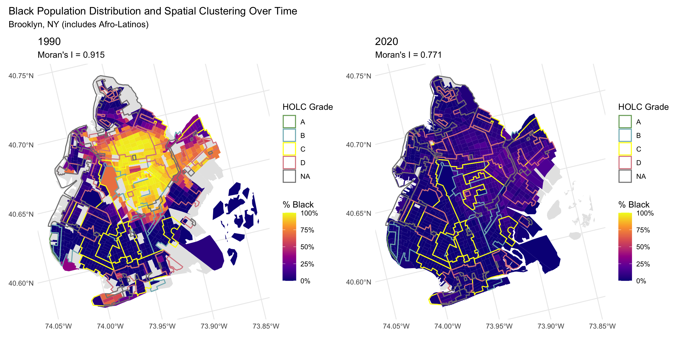
This analysis reveals that 1930s redlining policies continue to structure Brooklyn’s racial geography nearly a century later, though the nature of this structuring has evolved over time.
The Global Moran’s I statistics demonstrate extremely high spatial autocorrelation of Black populations in both time periods. In 1990, sixty years after redlining, the Moran’s I of 0.9154 indicated near-maximum clustering—Black residents were concentrated in specific neighborhoods to a degree that would almost never occur by random chance. By 2020, while the Moran’s I decreased to 0.7711, this still represents very strong clustering. Both values are statistically significant (p < 0.001), and the Monte Carlo simulations confirm these patterns are systematic rather than random.
To contextualize these values: Moran’s I ranges from -1 (perfect dispersion) to +1 (perfect clustering), with 0 indicating random distribution. A value of 0.77 in 2020 means that Brooklyn’s Black population remains profoundly spatially segregated, with similar values clustering together far more than would be expected under spatial randomness.
The decrease in Moran’s I from 0.91 to 0.77 over thirty years (1990-2020) might initially suggest progress toward residential integration. However, a critical interpretation reveals a more troubling dynamic: gentrification-driven displacement.
The same neighborhoods that were systematically disinvested through redlining—including parts of Bed-Stuy, Crown Heights, Bushwick, and East New York—have become targets for “revitalization” and development since the 1990s. This has led to dramatic increases in property values and rents, forcing long-time Black residents to relocate. This phenomenon represents what some scholars call “second-wave redlining” or “greenlined displacement”—where market forces accomplish what discriminatory lending policies once did: the removal of Black communities from specific urban spaces.
The decreasing clustering metric, therefore, may not reflect genuine integration but rather the displacement of Black residents from historically Black neighborhoods through economic pressure. This represents a continuation of spatial violence against Black communities—first through deliberate policy-based disinvestment, now through market-based displacement.
A critical methodological decision in this analysis was the inclusion of Hispanic Black populations (Afro-Latinos) in the demographic counts. New York City, and Brooklyn specifically, has substantial Caribbean and Latin American populations, including many who identify as both Black and Hispanic. Initial analysis using only Non-Hispanic Black populations (CV4AB) showed virtually no spatial clustering (Moran’s I ≈ 0, p > 0.05). Only when including Hispanic Black populations (CV4AG) did the strong clustering patterns emerge.
This finding underscores how measurement choices can obscure or reveal racial inequality. Excluding Afro-Latinos from analyses of Black spatial patterns systematically undercounts the Black diaspora in areas with significant Caribbean and Latin American communities, potentially leading to false conclusions about the absence of segregation. This has profound implications for how we understand and measure racial geography in diverse urban areas.
The LISA analysis identified 337 significant clusters (43.7% of tracts), revealing specific geographic concentrations of high and low Black population percentages. Visual inspection of the LISA maps suggests substantial correspondence between areas of significant clustering and historical D-grade redlining zones, particularly in East New York and central Brooklyn. This local-scale analysis confirms that redlining’s effects are not just visible in global statistics but manifest in specific, identifiable neighborhoods.
While Black population clustering decreased slightly over time, income clustering (Moran’s I = 0.59) remained highly significant in 2020. This suggests that even as some racial residential patterns shift (potentially through displacement), economic segregation persists. The spatial distribution of income continues to follow patterns established by mid-century discriminatory policies, creating lasting geographies of opportunity and disadvantage.
This spatial analysis demonstrates that the 1930s HOLC redlining policies in Brooklyn have created lasting geographic patterns that persist nearly a century later. Three key findings emerge from this research:
First, Brooklyn’s Black population exhibits extremely high spatial clustering in both 1990 (Moran’s I = 0.92) and 2020 (Moran’s I = 0.77), with both patterns statistically significant at p < 0.001. Monte Carlo simulations confirm these patterns are systematic rather than random, providing strong evidence that historical redlining established spatial structures that endure across generations.
Second, the modest decrease in clustering over thirty years (1990-2020) should not be interpreted as straightforward progress toward integration. Instead, this change likely reflects gentrification-driven displacement, where rising property values in historically disinvested neighborhoods force long-time Black residents to relocate. This represents a continuation of spatial injustice—what was accomplished through discriminatory policy in the 1930s is now achieved through market forces in the 2000s-2020s.
Third, methodological choices profoundly shape our understanding of racial geography. Including Afro-Latino populations in the analysis was essential for revealing the true extent of segregation in Brooklyn. This finding has important implications for how researchers measure and interpret racial patterns in diverse urban areas with significant Caribbean and Latin American populations.
These findings illuminate how racial injustice operates spatially and temporally. Redlining was not merely a historical wrong but an intervention that fundamentally restructured urban geography in ways that constrain residential choice, concentrate poverty, and limit access to opportunity generations later. Understanding these persistent spatial legacies is essential for developing policies that address—rather than reproduce—patterns of racial and economic inequality.
The spatial patterns documented here represent what geographer Ruth Wilson Gilmore calls “organized abandonment”—the systematic withdrawal of resources and investment from Black communities. Brooklyn’s contemporary geography reflects both this historical disinvestment and its ongoing manifestations through displacement and gentrification. Addressing these patterns requires policies that recognize housing as a site of ongoing racial violence and that center the needs of communities facing displacement rather than those seeking to profit from “revitalization.”
To further explore these patterns, future research could: