import pandas as pd
import numpy as np
import matplotlib.pyplot as plt
import seaborn as sns
from functools import reduce
from sklearn.preprocessing import StandardScaler
from scipy.stats import pearsonr
from sklearn.preprocessing import LabelEncoder
from sklearn.preprocessing import MinMaxScaler
from scipy.stats import pearsonr
from scipy.stats import f_onewayExploratory Data Analysis
Code
Cleaning (Continued)
I finished my data cleaning process with multiple DataFrames, so I am reading them to start working with the cleaned data. I also set up my processed_data_path variable to make it easier to reference the folder where my processed data is stored.
attendance_df = pd.read_csv('/Users/anilechoice/Documents/georgetown/5000/project-anilechoice00/data/processed-data/attendance_df.csv')
crime_df = pd.read_csv('/Users/anilechoice/Documents/georgetown/5000/project-anilechoice00/data/processed-data/crime_df.csv')
demo_df = pd.read_csv('/Users/anilechoice/Documents/georgetown/5000/project-anilechoice00/data/processed-data/demo_df.csv')
discipline_df = pd.read_csv('/Users/anilechoice/Documents/georgetown/5000/project-anilechoice00/data/processed-data/discipline_df.csv')
econ_df = pd.read_csv('/Users/anilechoice/Documents/georgetown/5000/project-anilechoice00/data/processed-data/econ_df.csv')
grad_df = pd.read_csv('/Users/anilechoice/Documents/georgetown/5000/project-anilechoice00/data/processed-data/grad_df.csv')
grocery_df = pd.read_csv('/Users/anilechoice/Documents/georgetown/5000/project-anilechoice00/data/processed-data/grocery_df.csv')
housing_df = pd.read_csv('/Users/anilechoice/Documents/georgetown/5000/project-anilechoice00/data/processed-data/housing_df.csv')
poverty_df = pd.read_csv('/Users/anilechoice/Documents/georgetown/5000/project-anilechoice00/data/processed-data/poverty_df.csv')
test_df = pd.read_csv('/Users/anilechoice/Documents/georgetown/5000/project-anilechoice00/data/processed-data/test_df.csv')

processed_data_path = '/Users/anilechoice/Documents/georgetown/5000/project-anilechoice00/data/processed-data/'
I put all my DataFrames in a list, then looped through to standardize all the column names. I stripped any extra spaces, converted the names to lowercase, and replaced underscores and colons with spaces. After that, I printed all the column names to ensure they looked the way I wanted.
# List of all your dataframes
dataframes = [attendance_df, crime_df, demo_df, discipline_df, econ_df, grad_df, grocery_df, housing_df, poverty_df, test_df]

# Standardize column names for all dataframes
for df in dataframes:
    df.columns = df.columns.str.strip().str.lower().str.replace('_', ' ').str.replace(':', '')

for i, df in enumerate(dataframes, start=1):
    print(f"DataFrame {i} columns:", df.columns)
DataFrame 1 columns: Index(['school name', 'student group', 'metric', 'metric score', 'metric n',
'ward', 'actual count'],
dtype='object')
DataFrame 2 columns: Index(['offense', 'ward'], dtype='object')
DataFrame 3 columns: Index(['ward', 'total population', 'black population', 'white population'], dtype='object')
DataFrame 4 columns: Index(['school name', 'student group', 'metric', 'metric score', 'metric n',
'ward'],
dtype='object')
DataFrame 5 columns: Index(['median household income', 'ward'], dtype='object')
DataFrame 6 columns: Index(['school name', 'graduates', 'cohort total', '2020 acgr', 'ward',
'actual count'],
dtype='object')
DataFrame 7 columns: Index(['store name', 'ward'], dtype='object')
DataFrame 8 columns: Index(['median home value', 'median gross rent', 'ward'], dtype='object')
DataFrame 9 columns: Index(['ward', 'poverty rate'], dtype='object')
DataFrame 10 columns: Index(['school name', 'student group', 'metric', 'metric score', 'metric n',
'ward', 'actual count'],
dtype='object')I wanted to see which DataFrames had missing values, so I used isna().sum() to count them for each. I noticed a few missing values - some in columns that I decided I wouldn’t be using but some in columns that I will need, which I will address later.
print(attendance_df.isna().sum())
print(crime_df.isna().sum())
print(demo_df.isna().sum())
print(discipline_df.isna().sum())
print(econ_df.isna().sum())
print(grad_df.isna().sum())
print(grocery_df.isna().sum())
print(housing_df.isna().sum())
print(poverty_df.isna().sum())
print(test_df.isna().sum())
school name 0
student group 0
metric 0
metric score 0
metric n 8
ward 4
actual count 0
dtype: int64
offense 0
ward 0
dtype: int64
ward 0
total population 0
black population 0
white population 0
dtype: int64
school name 0
student group 0
metric 0
metric score 0
metric n 0
ward 14
dtype: int64
median household income 0
ward 0
dtype: int64
school name 0
graduates 0
cohort total 0
2020 acgr 0
ward 5
actual count 0
dtype: int64
store name 0
ward 0
dtype: int64
median home value 0
median gross rent 0
ward 0
dtype: int64
ward 0
poverty rate 0
dtype: int64
school name 0
student group 0
metric 0
metric score 0
metric n 22
ward 8
actual count 0
dtype: int64I printed the rows in the graduation rate DataFrame where any values were missing so that I could look closer at the missing values. I noticed ‘State’ and ‘DCPS’ rows were missing ward values, and a few schools were missing the number of graduates.
# Find rows with missing values
missing_rows = grad_df[grad_df.isnull().any(axis=1)]

# Print the rows with missing values
print(missing_rows)
school name graduates cohort total \
0 State 3405 4802
1 DCPS 2180 3174
22 PCS 1223 1597
39 KIPP DC - College Preparatory Academy PCS 138 160
40 SEED PCS of Washington DC 28 35
2020 acgr ward actual count
0 0.71 NaN 3409
1 0.69 NaN 2190
22 0.77 NaN 1230
39 0.86 NaN 138
40 0.80 NaN 28 I noticed the poverty rate DataFrame included a row for the District of Columbia, which I wasn’t planning to analyze. It was also inconsistent with my other DataFrames, as they don’t have a row for the entire District. I dropped it here to avoid any issues when merging the DataFrames later.
After dropping the row, I printed the head of the DataFrame to make sure it was removed.
# Print head of poverty_df
print(poverty_df.head())

# Drop the "District of Columbia" row in the original poverty_df
poverty_df = poverty_df[poverty_df['ward'] != 'District of Columbia']

# Verify the result
print(poverty_df.head())
ward poverty rate
0 District of Columbia 0.079
1 Ward 1 0.063
2 Ward 2 0.043
3 Ward 3 0.042
4 Ward 4 0.091
ward poverty rate
1 Ward 1 0.063
2 Ward 2 0.043
3 Ward 3 0.042
4 Ward 4 0.091
5 Ward 5 0.102I started by renaming columns in the attendance_df. discipline_df, test_df, and grad_df DataFrames to make the column names more descriptive and unique to their respective DataFrames =. For example, I added prefixes like ‘attendance,’ ‘discipline,’ or ‘test’ to distinguish similar metrics across the datasets.
Next, I filtered out rows where the ‘school name’ was ‘State,’ ‘DCPS,’ or ‘PCS,’ as these rows weren’t relevant to my analysis. I also removed a few schools, like Ballou STAY High School and Duke Ellington School of the Arts, which are the rows that I saw were missing values a couple of cells back.
attendance_df = attendance_df.rename(columns={
    'metric score': 'attendance metric score',
    'metric n': 'attendance metric n',
    'metric': 'attendance metric',
    'student group': 'attendance student group',
    'actual count': 'attendance count'
})
# Filter out rows where 'school name' is 'State', 'DCPS', or 'PCS'
filtered_grad = attendance_df[~attendance_df['school name'].isin(['State', 'DCPS', 'PCS', 'Ballou STAY High School', 'Washington Metropolitan High School', 'Benjamin Banneker High School', 'Duke Ellington School of the Arts', 'KIPP DC - Somerset College Preparatory'])]


discipline_df = discipline_df.rename(columns={
    'metric score': 'discipline metric score',
    'metric n': 'discipline metric n',
    'metric': 'discipline metric',
    'student group': 'discipline student group'
})
# Filter out rows where 'school name' is 'State', 'DCPS', or 'PCS' and schools with missing values
discipline_df = discipline_df[~discipline_df['school name'].isin(['State', 'DCPS', 'PCS', 'Ballou STAY High School', 'Washington Metropolitan High School', 'Benjamin Banneker High School', 'Duke Ellington School of the Arts', 'KIPP DC - Somerset College Preparatory'])]


test_df = test_df.rename(columns={
    'metric score': 'test metric score',
    'metric n': 'test metric n',
    'metric': 'test metric',
    'student group': 'test student group',
    'actual count': 'test count'
})
# Filter out rows where 'school name' is 'State', 'DCPS', or 'PCS' and schools with missing values
test_df = test_df[~test_df['school name'].isin(['State', 'DCPS', 'PCS', 'Ballou STAY High School', 'Washington Metropolitan High School', 'Benjamin Banneker High School', 'Duke Ellington School of the Arts', 'KIPP DC - Somerset College Preparatory'])]


grad_df = grad_df.rename(columns={
    '2020 acgr': 'graduate rate'
})
# Filter out rows where 'school name' is 'State', 'DCPS', or 'PCS' and schools with missing values
grad_df = grad_df[~grad_df['school name'].isin(['State', 'DCPS', 'PCS', 'Ballou STAY High School', 'Washington Metropolitan High School', 'Benjamin Banneker High School', 'Duke Ellington School of the Arts', 'KIPP DC - Somerset College Preparatory'])]
To prepare to merge the data for analysis, I filtered and transformed each DataFrame into a standardized format using the melt() function. This helped consolidate indicators so that I could compare across wards. I focused on “All Report Card Students” for the DataFrames since a lot of the other demographic groups did not have values for analysis. It was easier to analyze the schools as a whole instead of by demographic since all DataFrames had a row for all students.
Attendance Data: I filtered to focus on ’In-Seat Attendance”. Then, I melted the data to create columns for indicators and their schools, grouped by ward.
Discipline Data: I calculated the total discipline metric scores for each school in each ward using groupby(), then melted the summary to align it with the format of the attendance data.
Test Data: I filtered test_df to include only “AP/IB Participation” for all students, then melted it like the others.
Graduation Data: I selected the relevant columns, including graduation rates, school names, wards, and counts. Then, I melted the data to focus on graduation rates by ward.
Grocery Data: I counted the number of grocery stores in each ward using group by () and melted the results into the same structure as the others.
Crime: I calculated the total number of crimes in each ward and melted the data.
Finally, I printed the head of each melted DataFrame to ensure that the transformations worked as I intended. This process puts all the DataFrames in a consistent format so that they are ready to be merged and analyzed.
# filter the attendance df
filtered_attendance = attendance_df[
    (attendance_df['attendance metric'] == 'In-Seat Attendance') &
    (attendance_df['attendance student group'] == 'All Report Card Students')
]

melted_attendance = filtered_attendance.melt(
    id_vars=['ward'],
    value_vars='attendance metric score',
    var_name='indicator',
    value_name='score')

# sum the Metric Score for each School Name
discipline_summary = discipline_df.groupby(['school name', 'ward'], as_index=False)['discipline metric score'].sum()

# Melt the discipline_summary DataFrame
melted_discipline = discipline_summary.melt(
    id_vars=['ward'],  # Columns to keep
    value_vars=['discipline metric score'],  # Columns to melt
    var_name='indicator',  # Name of the new 'indicator' column
    value_name='score'  # Name of the new 'value' column
)


# Filter for 'All Report Card Students' and 'AP/IB Participation'
filtered_test = test_df[
    (test_df['test student group'] == 'All Report Card Students') &
    (test_df['test metric'] == 'AP/IB Participation')
]

melted_test = filtered_test.melt(
    id_vars=['ward'],
    value_vars=['test metric score'],
    var_name='indicator',
    value_name='score'
)


filtered_grad = grad_df[['graduate rate','school name', 'ward', 'actual count']]

# Display the cleaned DataFrame
print(filtered_grad.head())


melted_grad = filtered_grad.melt(
    id_vars=['ward'],
    value_vars=['graduate rate'],
    var_name='indicator',
    value_name='score'
)

# Count the number of grocery stores by ward
grocery_counts = grocery_df.groupby('ward').size().reset_index(name='grocery store count')

melted_grocery = grocery_counts.melt(
    id_vars=['ward'],
    value_vars=['grocery store count'],
    var_name='indicator',
    value_name='score'
)

# Count the number of crimes by ward
crime_counts = crime_df.groupby('ward').size().reset_index(name='crime count')

melted_crime = crime_counts.melt(
    id_vars=['ward'],
    value_vars=['crime count'],
    var_name='indicator',
    value_name='score'
)

# Display the results
print("Melted Attendance:")
print(melted_attendance.head())
print("\nMelted Discipline:")
print(melted_discipline.head())
print("\nMelted Test:")
print(melted_test.head())
print("\nMelted Grad Rate:")
print(melted_grad.head())
print("\nMelted Grocery Count:")
print(melted_grocery.head())
print("\nMelted Crime Count:")
print(melted_crime.head())
graduate rate school name ward \
2 0.69 Roosevelt High School Ward 4
3 0.79 H.D. Woodson High School Ward 7
4 0.80 Dunbar High School Ward 5
5 0.99 School Without Walls High School Ward 2
6 0.93 Phelps Architecture, Construction and Engineer... Ward 5
actual count
2 163
3 107
4 136
5 147
6 66
Melted Attendance:
ward indicator score
0 Ward 8 attendance metric score 0.61
1 Ward 8 attendance metric score 0.61
2 Ward 2 attendance metric score 0.96
3 Ward 1 attendance metric score 0.77
4 Ward 1 attendance metric score 0.87
Melted Discipline:
ward indicator score
0 Ward 8 discipline metric score 96
1 Ward 2 discipline metric score 47
2 Ward 8 discipline metric score 9
3 Ward 4 discipline metric score 105
4 Ward 1 discipline metric score 288
Melted Test:
ward indicator score
0 Ward 8 test metric score 0.23
1 Ward 8 test metric score 0.19
2 Ward 1 test metric score 0.44
3 Ward 1 test metric score 0.98
4 Ward 4 test metric score 0.38
Melted Grad Rate:
ward indicator score
0 Ward 4 graduate rate 0.69
1 Ward 7 graduate rate 0.79
2 Ward 5 graduate rate 0.80
3 Ward 2 graduate rate 0.99
4 Ward 5 graduate rate 0.93
Melted Grocery Count:
ward indicator score
0 Ward 1 grocery store count 14
1 Ward 2 grocery store count 17
2 Ward 3 grocery store count 16
3 Ward 4 grocery store count 12
4 Ward 5 grocery store count 11
Melted Crime Count:
ward indicator score
0 Ward 1 crime count 105
1 Ward 2 crime count 183
2 Ward 3 crime count 68
3 Ward 4 crime count 92
4 Ward 5 crime count 173Since these DataFrames were straightforward and included only the rows I needed, all I had to do was melt them. Like in the previous cell, I used the ‘ward’ column as the identifier. Each data frame was melted to focus on its specific indicator.
Demographics Data: Total population, Black population, and White population were included.
Economic Data: Focused on median household income.
Housing: Focused on median home value and gross median rent
Poverty Data: Focused on poverty data.
Lastly, I printed the heads of the melted DataFrames to confirm everything looked correct.
melted_demo = demo_df.melt(
    id_vars=['ward'],
    value_vars=['total population', 'black population', 'white population'],
    var_name='indicator',
    value_name='score'
)

melted_econ = econ_df.melt(
    id_vars=['ward'],
    value_vars='median household income',
    var_name='indicator',
    value_name='score'
)

melted_housing = housing_df.melt(
    id_vars=['ward'],
    value_vars=['median home value', 'median gross rent'],
    var_name='indicator',
    value_name='score'
)

melted_poverty = poverty_df.melt(
    id_vars=['ward'],
    value_vars=['poverty rate'],
    var_name='indicator',
    value_name='score'
)

# Display the results
print("Melted Demographic:")
print(melted_demo.head())
print("\nMelted Economic:")
print(melted_econ.head())
print("\nMelted Housing:")
print(melted_housing.head())
print("\nMelted Poverty:")
print(melted_poverty.head())
Melted Demographic:
ward indicator score
0 Ward 1 total population 79448
1 Ward 2 total population 77904
2 Ward 3 total population 79851
3 Ward 4 total population 86071
4 Ward 5 total population 89628
Melted Economic:
ward indicator score
0 Ward 1 median household income 118395
1 Ward 2 median household income 128048
2 Ward 3 median household income 141393
3 Ward 4 median household income 115068
4 Ward 5 median household income 92398
Melted Housing:
ward indicator score
0 Ward 1 median home value 783300
1 Ward 2 median home value 741700
2 Ward 3 median home value 1118400
3 Ward 4 median home value 792700
4 Ward 5 median home value 671600
Melted Poverty:
ward indicator score
0 Ward 1 poverty rate 0.063
1 Ward 2 poverty rate 0.043
2 Ward 3 poverty rate 0.042
3 Ward 4 poverty rate 0.091
4 Ward 5 poverty rate 0.102To accurately represent the scores across wards, I calculated weighted averages for attendance, test scores, and graduation rates. This approach ensures that scores are weighted by the number of students or counts rather than treating each school equally regardless of size.
Attendance: I grouped the data by ward and calculated a weighted average of the attendance metric score using the attendance count as weights.
Test Scores: I calculated the weighted average of the test metric scores using the test count as weights.
Graduation Rates: For graduation rates, I weighted the scores by the actual number of graduates in each school.
For each calculation, I used groupby(‘ward’) and a lambda function to compute the weighted sum for each group. The results were then reset into a clean DataFrame with descriptive column names like ‘weighted attendance score,’ ‘weighted test score’, and ‘weighted grad score.’
# Weighted average for attendance
attendance_aggregated = (
    filtered_attendance
    .groupby('ward')
    .apply(lambda group:
        (group['attendance metric score'] * group['attendance count']).sum() / group['attendance count'].sum()
    )
    .reset_index(name='weighted attendance score')
)

# Weighted average for test scores
test_aggregated = (
    filtered_test
    .groupby('ward')
    .apply(lambda group:
        (group['test metric score'] * group['test count']).sum() / group['test count'].sum()
    )
    .reset_index(name='weighted test score')
)

grad_aggregated = (
    filtered_grad
    .groupby('ward')
    .apply(lambda group:
        (group['graduate rate'] * group['actual count']).sum() / group['actual count'].sum()
    )
    .reset_index(name='weighted grad score')
)
/var/folders/ph/mfm_2j1s57n8ylwflpqw64840000gn/T/ipykernel_72077/2996669866.py:5: DeprecationWarning: DataFrameGroupBy.apply operated on the grouping columns. This behavior is deprecated, and in a future version of pandas the grouping columns will be excluded from the operation. Either pass `include_groups=False` to exclude the groupings or explicitly select the grouping columns after groupby to silence this warning.
.apply(lambda group:
/var/folders/ph/mfm_2j1s57n8ylwflpqw64840000gn/T/ipykernel_72077/2996669866.py:15: DeprecationWarning: DataFrameGroupBy.apply operated on the grouping columns. This behavior is deprecated, and in a future version of pandas the grouping columns will be excluded from the operation. Either pass `include_groups=False` to exclude the groupings or explicitly select the grouping columns after groupby to silence this warning.
.apply(lambda group:
/var/folders/ph/mfm_2j1s57n8ylwflpqw64840000gn/T/ipykernel_72077/2996669866.py:24: DeprecationWarning: DataFrameGroupBy.apply operated on the grouping columns. This behavior is deprecated, and in a future version of pandas the grouping columns will be excluded from the operation. Either pass `include_groups=False` to exclude the groupings or explicitly select the grouping columns after groupby to silence this warning.
.apply(lambda group:I merged the aggregated DataFrames for attendance, test scores, and graduation rates into a single DataFrame, aligning them by work. This combined the weighted scores for each indicator into one place.
To prepare the merged DataFrame, I used the melt() function. This transformed the wide format (with separate columns for each indicator) into a long format, with columns for ‘ward,’ ‘indicator,’ and ‘score.’ The long format makes it easier to work with the data for comparison and plotting.
Finally, I printed the head of the merged and melted DataFrames to confirm everything worked as I intended.
# Merge attendance and test aggregated data
aggregated_df = pd.merge(attendance_aggregated, test_aggregated, on='ward', how='outer')

# Merge the result with graduation aggregated data
aggregated_df = pd.merge(aggregated_df, grad_aggregated, on='ward', how='outer')

print(aggregated_df.head())

# Melt the merged DataFrame
aggregated_df = pd.melt(
    aggregated_df,
    id_vars=['ward'],  # Columns to keep
    var_name='indicator',  # Name for the new column that holds variable names
    value_name='score'  # Name for the new column that holds values
)

print(aggregated_df.head())
ward weighted attendance score weighted test score weighted grad score
0 Ward 1 0.846135 0.798017 0.724455
1 Ward 2 0.938432 0.982184 0.980154
2 Ward 3 0.880000 0.820000 0.870000
3 Ward 4 0.883593 0.611682 0.793011
4 Ward 5 0.856182 0.845709 0.862886
ward indicator score
0 Ward 1 weighted attendance score 0.846135
1 Ward 2 weighted attendance score 0.938432
2 Ward 3 weighted attendance score 0.880000
3 Ward 4 weighted attendance score 0.883593
4 Ward 5 weighted attendance score 0.856182I combined the melted DataFrames (attendance, discipline, grocery, crime, demographics, economic, housing, and poverty data) into a single list to bring all the data together. I concatenated them into one DataFrame using pd.concat().
Next, I created a pivot table (wardlevel_cat_df) to organize the data at the ward level. This table uses ‘ward’ as the index, ‘indicator’ as columns, and ‘score’ as the values which structured the data in a way that lets me see all the indicators for each ward in a clean and organized format.
Finally, I printed the resulting pivot table.
final_combined_df = [
    aggregated_df,
    melted_discipline,
    melted_grocery,
    melted_crime,
    melted_demo,
    melted_econ,
    melted_housing,
    melted_poverty
]

cat_df = pd.concat(final_combined_df, ignore_index=True)

wardlevel_cat_df = cat_df.pivot_table(
    index='ward',
    columns='indicator',
    values='score'
).reset_index()

print(wardlevel_cat_df)
indicator ward black population crime count discipline metric score \
0 Ward 1 18058.0 105.0 162.250000
1 Ward 2 8458.0 183.0 39.500000
2 Ward 3 6599.0 68.0 278.000000
3 Ward 4 40887.0 92.0 104.428571
4 Ward 5 52894.0 173.0 137.333333
5 Ward 6 18470.0 134.0 41.000000
6 Ward 7 74989.0 129.0 118.166667
7 Ward 8 71525.0 116.0 55.200000
indicator grocery store count median gross rent median home value \
0 14.0 2003.0 783300.0
1 17.0 2329.0 741700.0
2 16.0 2079.0 1118400.0
3 12.0 1560.0 792700.0
4 11.0 1608.0 671600.0
5 12.0 2392.0 848000.0
6 4.0 1190.0 449000.0
7 4.0 1288.0 392700.0
indicator median household income poverty rate total population \
0 118395.0 0.063 79448.0
1 128048.0 0.043 77904.0
2 141393.0 0.042 79851.0
3 115068.0 0.091 86071.0
4 92398.0 0.102 89628.0
5 133590.0 0.069 80772.0
6 62243.0 0.130 89870.0
7 48609.0 0.170 87043.0
indicator weighted attendance score weighted grad score \
0 0.846135 0.724455
1 0.938432 0.980154
2 0.880000 0.870000
3 0.883593 0.793011
4 0.856182 0.862886
5 0.900000 0.677576
6 0.794396 0.798904
7 0.775443 0.692264
indicator weighted test score white population
0 0.798017 36131.0
1 0.982184 47709.0
2 0.820000 55750.0
3 0.611682 21551.0
4 0.845709 21057.0
5 0.180000 47680.0
6 0.545874 5987.0
7 0.287179 7865.0 I set the file path for the wardlevel_cat_df DataFrame, and then I used .to_csv() to save it in my processed data folder for future analysis. This DataFrame will serve as the DataFrame that still contains the categorical values and is not normalized.
wardlevel_cat_path = processed_data_path + 'wardlevel_cat_df.csv'
wardlevel_cat_df.to_csv(wardlevel_cat_path, index=False)
I decided to create another DataFrame with normalized indicators, and I also encoded the wards numerically.
Normalization: I used the StandardScaler to normalize the scores for specific indicators, such as grocery store counts, crime counts, median household income, and weighted scores for attendance, tests, and graduation rates. I normalized these scores to ensure all indicators are on the same scale, essential for clustering and machine learning.
I applied the normalization separately for each indicator using a groupby() operation on the ‘indicator’ column. I did this so that each was scaled independently, and the normalized scores were added as a new column called ‘normalized score.’
Encoded Wards: I numerically encoded the ‘ward’ column using the LabelEncoder in order to assign a unique integer to each ward. This is another essential step for algorithms that require numeric inputs.
Finally, I printed the head of the resulting DataFrame to check that the normalization and encoding were correctly applied.
# Initialize Min-Max Scaler
scaler = StandardScaler()

final_df = pd.concat(final_combined_df, ignore_index=True)

# Apply normalization to each indicator separately
def normalize_group(group):
    group['normalized score'] = scaler.fit_transform(group[['score']]).flatten()
    return group

final_df = final_df.groupby('indicator', group_keys=False).apply(normalize_group)


# Encode ward numerically
label_encoder = LabelEncoder()
final_df['ward encoded'] = label_encoder.fit_transform(final_df['ward'])

print(final_df.head())
ward indicator score normalized score ward encoded
0 Ward 1 weighted attendance score 0.846135 -0.260389 0
1 Ward 2 weighted attendance score 0.938432 1.568955 1
2 Ward 3 weighted attendance score 0.880000 0.410822 2
3 Ward 4 weighted attendance score 0.883593 0.482027 3
4 Ward 5 weighted attendance score 0.856182 -0.061260 4/var/folders/ph/mfm_2j1s57n8ylwflpqw64840000gn/T/ipykernel_72077/2675682030.py:11: DeprecationWarning: DataFrameGroupBy.apply operated on the grouping columns. This behavior is deprecated, and in a future version of pandas the grouping columns will be excluded from the operation. Either pass `include_groups=False` to exclude the groupings or explicitly select the grouping columns after groupby to silence this warning.
final_df = final_df.groupby('indicator', group_keys=False).apply(normalize_group)To organize the normalized data, I created a pivot table (wardlevel_df), which uses the encoded ward values (ward encoded) as the index and the indicators as columns, with their normalized scores as the values - this structure provides a clean, ward-level view of all the indicators, making it easier to analyze relationships and patterns across wards.
Then, I printed the wardlevel_df to confirm that the pivot table was created successfully.
wardlevel_df = final_df.pivot_table(
    index='ward encoded',
    columns='indicator',
    values='normalized score'
).reset_index()

print(wardlevel_df)
indicator ward encoded black population crime count \
0 0 -0.713111 -0.549857
1 1 -1.084623 1.594586
2 2 -1.156565 -1.567094
3 3 0.170354 -0.907265
4 4 0.635016 1.319658
5 5 -0.697167 0.247436
6 6 1.490075 0.109971
7 7 1.356021 -0.247436
indicator discipline metric score grocery store count median gross rent \
0 0.618471 0.597438 0.458071
1 -0.832808 1.249189 1.216580
2 1.986988 1.031938 0.634902
3 -0.065155 0.162938 -0.572662
4 0.323880 -0.054313 -0.460980
5 -0.815074 0.162938 1.363162
6 0.097271 -1.575064 -1.433545
7 -0.647186 -1.575064 -1.205528
indicator median home value median household income poverty rate \
0 0.273488 0.421431 -0.619639
1 0.079422 0.724407 -1.100912
2 1.836742 1.143264 -1.124976
3 0.317339 0.317007 0.054143
4 -0.247597 -0.394532 0.318844
5 0.575316 0.898353 -0.475257
6 -1.286034 -1.341001 0.992626
7 -1.548676 -1.768928 1.955172
indicator total population weighted attendance score weighted grad score \
0 -0.963581 -0.260389 -0.786304
1 -1.303614 1.568955 1.878423
2 -0.874829 0.410822 0.730472
3 0.494991 0.482027 -0.071855
4 1.278343 -0.061260 0.656333
5 -0.671999 0.807226 -1.274848
6 1.331638 -1.285860 -0.010446
7 0.709053 -1.661521 -1.121775
indicator weighted test score white population
0 0.619341 0.317723
1 1.314056 0.967106
2 0.702267 1.418107
3 -0.083549 -0.500036
4 0.799246 -0.527743
5 -1.711937 0.965480
6 -0.331788 -1.372985
7 -1.307635 -1.267652 I again used the processed data path in order to save the ward level DataFrame to my processed data folder.
wardlevel_file_path = processed_data_path + 'wardlevel_df.csv'
wardlevel_df.to_csv(wardlevel_file_path, index=False)
I started by selecting the relevant columns (school name, scores, and wards) from each filtered DataFrame for attendance, test scores, graduation rates, and discipline metrics to analyze student success indicators at the school level. This gave me the key information necessary for analysis.
Next, I merged these DataFrames into a single student_success_df using a list of the selected DataFrames and the reduce() function. The merge was performed on ‘school name’ and ‘ward’ to align the data across schools.
After merging, I dropped rows with missing values (NaN) to ensure the final DataFrame was clean and ready for analysis. Finally, I printed the DataFrame’s info and previewed the first few rows to verify that the merge and cleaning steps worked as I intended.
# print(filtered_attendance.columns.unique)
ml_attendance = filtered_attendance[['school name','attendance metric score','ward']]
# print(ml_attendance)

# print(filtered_test.columns.unique)
ml_test = filtered_test[['school name', 'test metric score', 'ward']]
# print(ml_test)

# print(filtered_grad.columns.unique)
ml_grad = filtered_grad[['school name', 'graduate rate', 'ward']]
# print(ml_grad)

print(discipline_summary.columns.unique)
ml_discipline = discipline_summary[['school name', 'discipline metric score', 'ward']]
# print(ml_discipline)


# List of all student indicator DataFrames
dfs_to_merge = [ml_attendance, ml_test, ml_grad, ml_discipline]

# Merge all DataFrames
student_success_df = reduce(lambda left, right: pd.merge(left, right, on=['school name', 'ward'], how='outer'), dfs_to_merge)

# print(student_success_df.head())

# Drop rows with NaN values
student_success_df = student_success_df.dropna()

# Verify the result
print(student_success_df.info())
print(student_success_df.head())
<bound method Index.unique of Index(['school name', 'ward', 'discipline metric score'], dtype='object')>
<class 'pandas.core.frame.DataFrame'>
Index: 28 entries, 0 to 36
Data columns (total 6 columns):
# Column Non-Null Count Dtype
--- ------ -------------- -----
0 school name 28 non-null object
1 attendance metric score 28 non-null float64
2 ward 28 non-null object
3 test metric score 28 non-null float64
4 graduate rate 28 non-null float64
5 discipline metric score 28 non-null float64
dtypes: float64(4), object(2)
memory usage: 1.5+ KB
None
school name attendance metric score ward \
0 Anacostia High School 0.61 Ward 8
1 BASIS DC PCS 0.96 Ward 2
2 Ballou High School 0.61 Ward 8
4 Capital City PCS - High School 0.91 Ward 4
5 Cardozo Education Campus 0.77 Ward 1
test metric score graduate rate discipline metric score
0 0.23 0.62 96.0
1 0.95 0.95 47.0
2 0.19 0.62 9.0
4 0.47 0.89 105.0
5 0.44 0.64 288.0 I calculated the number of unique grocery stores and the total number of crimes for each ward:
Grocery Store Counts: - I grouped the grocery_df by ‘ward’ and used .nunique() on the ‘store name’ column to count the unique stores in each ward. - Then, I reset the index to turn the result into a clean DataFrame. - To make the column name more descriptive, I renamed ‘store name’ to ‘grocery store count.’
Crime Counts: - I grouped the crime_df by ‘ward’ and used .count() on the ‘offense’ column to get the total number of crimes reported in each ward. - I reset the index and renamed the ‘offense’ column to ‘crime count’ for clarity.
grocery_store_counts = grocery_df.groupby('ward')['store name'].nunique().reset_index()

print(grocery_store_counts.columns)

grocery_store_counts.rename(columns={'store name': 'grocery store count'}, inplace=True)


crime_counts = crime_df.groupby('ward')['offense'].count().reset_index()

crime_counts.rename(columns={'offense': 'crime count'}, inplace=True)
Index(['ward', 'store name'], dtype='object')Here, I printed the DataFrames I just created to make sure they were correct.
print(grocery_store_counts)
print(crime_counts)
ward grocery store count
0 Ward 1 12
1 Ward 2 12
2 Ward 3 11
3 Ward 4 10
4 Ward 5 11
5 Ward 6 9
6 Ward 7 3
7 Ward 8 4
ward crime count
0 Ward 1 105
1 Ward 2 183
2 Ward 3 68
3 Ward 4 92
4 Ward 5 173
5 Ward 6 134
6 Ward 7 129
7 Ward 8 116I merged the socioeconomic DataFrames to have a single dataset with all the indicators aligned by ward. I started with demo_df and merged it with econ_df on the ‘ward’ column. Then, I added housing_df and poverty_df, and finally, grocery_store_counts and crime_counts.
The final socioeconomic_df contains each ward’s combined socioeconomic indicators (ie, demographics, economic indicators, housing, poverty rates, grocery store counts, and crime counts) into one DataFrame. Lastly, I printed the Dataframe to confirm all the columns were included and the data was merged correctly.
# Merging socioeconomic dataframes
socioeconomic_df = demo_df.merge(econ_df, on='ward')
socioeconomic_df = socioeconomic_df.merge(housing_df, on='ward')
socioeconomic_df = socioeconomic_df.merge(poverty_df, on='ward')
socioeconomic_df = socioeconomic_df.merge(grocery_store_counts, on='ward')
socioeconomic_df = socioeconomic_df.merge(crime_counts, on='ward')

print(socioeconomic_df)
ward total population black population white population \
0 Ward 1 79448 18058 36131
1 Ward 2 77904 8458 47709
2 Ward 3 79851 6599 55750
3 Ward 4 86071 40887 21551
4 Ward 5 89628 52894 21057
5 Ward 6 80772 18470 47680
6 Ward 7 89870 74989 5987
7 Ward 8 87043 71525 7865
median household income median home value median gross rent \
0 118395 783300 2003
1 128048 741700 2329
2 141393 1118400 2079
3 115068 792700 1560
4 92398 671600 1608
5 133590 848000 2392
6 62243 449000 1190
7 48609 392700 1288
poverty rate grocery store count crime count
0 0.063 12 105
1 0.043 12 183
2 0.042 11 68
3 0.091 10 92
4 0.102 11 173
5 0.069 9 134
6 0.130 3 129
7 0.170 4 116 Finally, I merged my student success DataFrame with the socioeconomic DataFrame on ‘ward.’ I now have a dataset organized at the school level while still including wards so that I can still group that way when necessary.
I printed the head of the final DataFrame to confirm that the merge worked as expected and that all the key indicators were included.
# Merge the student success data with socioeconomic data on 'ward'
final_df = student_success_df.merge(socioeconomic_df, on='ward')

print(final_df.head())
school name attendance metric score ward \
0 Anacostia High School 0.61 Ward 8
1 BASIS DC PCS 0.96 Ward 2
2 Ballou High School 0.61 Ward 8
3 Capital City PCS - High School 0.91 Ward 4
4 Cardozo Education Campus 0.77 Ward 1
test metric score graduate rate discipline metric score \
0 0.23 0.62 96.0
1 0.95 0.95 47.0
2 0.19 0.62 9.0
3 0.47 0.89 105.0
4 0.44 0.64 288.0
total population black population white population \
0 87043 71525 7865
1 77904 8458 47709
2 87043 71525 7865
3 86071 40887 21551
4 79448 18058 36131
median household income median home value median gross rent \
0 48609 392700 1288
1 128048 741700 2329
2 48609 392700 1288
3 115068 792700 1560
4 118395 783300 2003
poverty rate grocery store count crime count
0 0.170 4 116
1 0.043 12 183
2 0.170 4 116
3 0.091 10 92
4 0.063 12 105 EDA
Here, I plotted a graph to look at the relationship between graduation rates of the different schools and the median household income of their respective wards.
Interpretations:
Positive Correlation:
Higher median household incomes are generally associated with higher graduation rates.
Ward Differences:
Wards like Ward 8 and 7 have lower graduation rates and lower median household incomes which reflect potential socioeconomic disparities.
In contrast, Ward 2 and Ward 3 cluster at the higher end of both graduation rate and median household income.
The clustering of points suggests distinct groupings based on ‘ward.’
sns.lmplot(data=final_df,
           x='graduate rate',
           y='median household income',
           hue='ward')
plt.title("Graduation Rate vs. Median Houshold Income by Ward")
plt.show()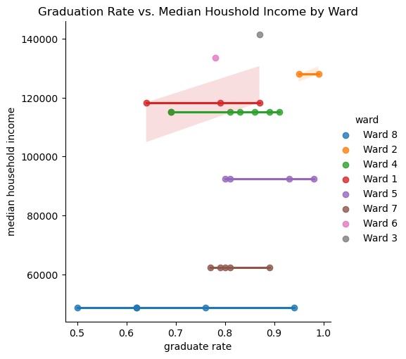
Similarly to the previous DataFrame, I wanted to normalize the data for consistent scaling across all indicators. This time, I was normalizing entire columns.
I created a list of the columns I wanted to normalize, which included all the indicators. Then, I used StandardScaler to apply normalization across all these columns in the final DataFrame.
I finished this by printing the head of the DataFame to ensure everything was normalized correctly.
# Initialize Min-Max Scaler
scaler = StandardScaler()

# List of columns to normalize
columns_to_normalize = [
    'grocery store count',
    'crime count',
    'median household income',
    'median home value',
    'median gross rent',
    'discipline metric score',
    'total population',
    'black population',
    'white population',
    'attendance metric score',
    'test metric score',
    'graduate rate',
    'discipline metric score'
]

# Apply normalization to each column
final_df[columns_to_normalize] = scaler.fit_transform(final_df[columns_to_normalize])


print(final_df.head())
school name attendance metric score ward \
0 Anacostia High School -2.402762 Ward 8
1 BASIS DC PCS 1.116979 Ward 2
2 Ballou High School -2.402762 Ward 8
3 Capital City PCS - High School 0.614159 Ward 4
4 Cardozo Education Campus -0.793738 Ward 1
test metric score graduate rate discipline metric score \
0 -1.071328 -1.610130 -0.234854
1 1.460674 1.234536 -0.800150
2 -1.211995 -1.610130 -1.238544
3 -0.227328 0.717324 -0.131024
4 -0.332828 -1.437726 1.980187
total population black population white population \
0 0.326186 1.034757 -0.954451
1 -1.938591 -1.667535 1.766317
2 0.326186 1.034757 -0.954451
3 0.085310 -0.278019 -0.019895
4 -1.555965 -1.256195 0.975707
median household income median home value median gross rent \
0 -1.460012 -1.365572 -0.860898
1 1.128581 0.475564 1.985455
2 -1.460012 -1.365572 -0.860898
3 0.705615 0.744613 -0.117182
4 0.814029 0.695023 1.094090
poverty rate grocery store count crime count
0 0.170 -1.168424 -0.219525
1 0.043 1.068558 1.881640
2 0.170 -1.168424 -0.219525
3 0.091 0.509313 -0.972181
4 0.063 1.068558 -0.564492 Next, I printed a correlation matrix for the DataFrame with schools.
Strong Positive Correlations:
Median Household Income has strong positive correlations with: - Median Home Value (0.97) - Median Gross Rent (0.84) These findings imply that wealthier wards tend to have high home values and rent costs, which could have significant implications for educational resources and opportunities. The strong correlation (0.93) between the Black Population and Poverty Rate highlights systemic disparities that need to be addressed for a more equitable education system.
Strong Negative Correlations:
The high negative correlation between the White and Black populations (0.97) reflects the racial divide across wards. This could indicate that certain wards are more racially homogenous, which may have implications for the diversity and inclusivity of the educational environment. Poverty rate shares a negative correlation with wealth indicators; Median Household Income (-0.95), Median Home Value (-0.90), and Median Gross Rent (-0.85).
Education Metrics:
Graduation rate correlates positively with the following: - Attendance metric Score (0.63) - Test Metric Score (0.59) - This indicates that higher attendance and test scores are associated with higher graduation rates. - Poverty rate has a moderate negative correlation with Graduation Rate (-0.45), suggesting that poverty may impact educational outcomes.
Grocery Store & Crime Counts:
Grocery Store Count has a moderate positive correlation with Test Metric Score (0.57) and Attendance Metric Score (0.39). This might reflect better resources in wards with more grocery stores, as those wards also have higher median household income values. While Crime Count did not show any substantially strong correlations with other indicators, it did have a minor positive correlation with Test Metric Score (0.27). This suggests that in areas with higher crime rates, there may be a slight negative impact on test scores, which could be due to factors such as safety concerns affecting student attendance and concentration.
Key Takeaway:
The matrix highlights significant relationships between socioeconomic factors and educational outcomes. This reinforces the interconnectedness of social and economic disparities with student success indicators. I also used this correlation matrix to identify potential issues with collinearity. Highly correlated features can introduce redundancy in machine learning models, so I dropped those columns to avoid this.
numeric_columns = final_df.select_dtypes(include=['float64', 'int64']).columns
numeric_df = final_df[numeric_columns]

plt.figure(figsize=(12, 8))
sns.heatmap(numeric_df.corr(), annot=True, fmt=".2f", cmap="coolwarm")
plt.title("Correlation Matrix")
plt.show()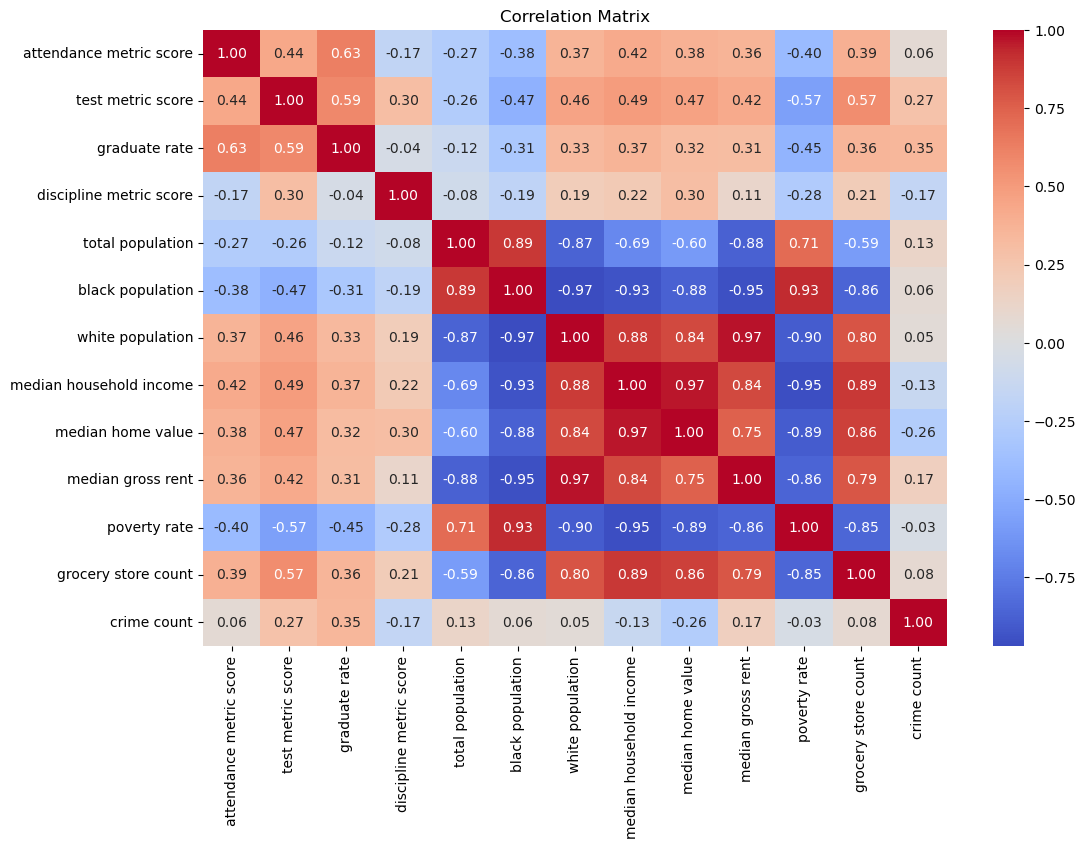
Based on the matrix, I selected the following features to drop: - Total Population: A high correlation exists between the Black population and the White population columns. - Median Home Value and Gross Rent: Both strongly correlated with Median Homehold Income. - Crime Count: Weak correlations with most indicators, contributing minimal unique information.
I dropped these columns in the cell to create a refined DataFrame (refined_df) for machine learning.
# Features to drop
features_to_drop = ['total population', 'median home value', 'median gross rent', 'crime count']

refined_df = final_df.drop(columns=features_to_drop)

print(refined_df.head())
school name attendance metric score ward \
0 Anacostia High School -2.402762 Ward 8
1 BASIS DC PCS 1.116979 Ward 2
2 Ballou High School -2.402762 Ward 8
3 Capital City PCS - High School 0.614159 Ward 4
4 Cardozo Education Campus -0.793738 Ward 1
test metric score graduate rate discipline metric score \
0 -1.071328 -1.610130 -0.234854
1 1.460674 1.234536 -0.800150
2 -1.211995 -1.610130 -1.238544
3 -0.227328 0.717324 -0.131024
4 -0.332828 -1.437726 1.980187
black population white population median household income poverty rate \
0 1.034757 -0.954451 -1.460012 0.170
1 -1.667535 1.766317 1.128581 0.043
2 1.034757 -0.954451 -1.460012 0.170
3 -0.278019 -0.019895 0.705615 0.091
4 -1.256195 0.975707 0.814029 0.063
grocery store count
0 -1.168424
1 1.068558
2 -1.168424
3 0.509313
4 1.068558 I then saved final_df to the processed data folder, which I’ll be using for my supervised and unsupervised learning.
final_df_path = processed_data_path + 'ml_df.csv'
refined_df.to_csv(final_df_path, index=False)
The following bar chart shows the number of schools in each ward. I also decided to show the proportion of the Black population per ward. First, I grouped grad_df by ward and calculated the average black proportion for each ward. This was so I could assign color to each bar based on the mean proportion.
‘mcolor.Normalize’ scales the Black proportion values to a range between 0 and 1 for the colormap since colormap requires values between 0 and 1. I then assigned a color from the coolwarm gradient based on the normalized value. Next, I created a dictionary where each ward is mapped to its corresponding color based on the Black population proportion. This is to assign a specific color to each ward in the chart.
‘bar_color’ counts the number of schools in each ward, sorted so that it ascends for wards 1 to 8, and then maps the ward names to their corresponding color using the ward_color_map. This ensures each bar in the chart is colored based on its ward’s Black population proportion.
Finally, I plotted the bar chart to show the frequency of schools in each ward, and color=bar_colors is what colors each bar based on the bar_color list.
I also added a legend so that we can see what each color is indicative of.
School Distribution:
- The color gradient indicates the proportion of the Black population, with blue shades representing lower proportions and red shades representing higher proportions.
- Wards 7 and 8 have high Black population proportions and higher numbers of schools.
Ward-Specific Patterns:
- Ward 4 has the highest school count but with a relatively neutral color, indicating a balanced demographic. Ward 5 is also close to neutral but leans more red.
- Wards 1, 2, 3, and 6 have fewer schools and lower Black population proportions, as represented by the blue colors.
import matplotlib.cm as cm
import matplotlib.colors as mcolors

# Calculate Black proportion
demo_df['black proportion'] = demo_df['black population'] / demo_df['total population']

# Merge it into grad_df
grad_df = grad_df.merge(
    demo_df[['ward', 'black proportion']],
    on='ward',
    how='left'
)

# Aggregate black proportion by ward
ward_black_proportion = grad_df.groupby('ward')['black proportion'].mean().reset_index()

# Normalize black proportion based on aggregated values
norm = mcolors.Normalize(vmin=ward_black_proportion['black proportion'].min(),
                         vmax=ward_black_proportion['black proportion'].max())
colors = [cm.coolwarm(norm(value)) for value in ward_black_proportion['black proportion']]

# Create a mapping of ward to color
ward_color_map = dict(zip(ward_black_proportion['ward'], colors))

# Map the colors to wards for the bar chart
bar_colors = grad_df['ward'].value_counts().sort_index().index.map(ward_color_map)

# Create a bar plot
fig, ax = plt.subplots(figsize=(10, 6))
grad_df['ward'].value_counts().sort_index().plot(
    kind='bar',
    color=bar_colors,
    ax=ax
)
ax.set_title("Frequency of Schools by Ward (Colored by Black Population Proportion)")
ax.set_xlabel("Ward")
ax.set_ylabel("School Count")

# Add a colorbar legend
sm = cm.ScalarMappable(cmap="coolwarm", norm=norm)
sm.set_array([])
cbar = fig.colorbar(sm, ax=ax, pad=0.02)
cbar.set_label("Black Population Proportion")

plt.show()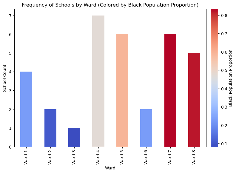
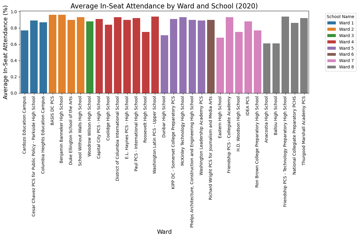
The following chart shows the average in-seat attendance for schools across each ward where bar represents a school and is color-coded in order to group by ward.
Overall Trend:
Some Schools are doing well, with attendance close to 100%, while others are struggling.
Differences Between Wards:
- Ward 2 and Ward 3 stand out with consistently higher attendance rates
- Ward 7 and Ward 8 seem to have more schools with lower attendance rates
School-Level Differences:
Even within the same ward, some schools have much higher attendance than others - for example, Wards 4 and 8 have a mix of attendance rates. This shows that issues could be school-specific in some cases.
# Aggregate attendance data by Ward
attendance_summary = filtered_attendance.groupby(['ward', 'school name'])['attendance metric score'].mean().reset_index()

# Plot a bar chart
plt.figure(figsize=(12, 8))
sns.barplot(
    data=attendance_summary,
    x='school name',  # school on the x-axis
    y='attendance metric score',  # Metric Score on the y-axis
    hue='ward',  # Different wards represented as colors
    dodge=False  # Avoid stacking
)

# Add labels and title
plt.xlabel('Ward', fontsize=14)
plt.ylabel('Average In-Seat Attendance (%)', fontsize=14)
plt.title('Average In-Seat Attendance by Ward and School (2020)', fontsize=16)
plt.xticks(rotation=90)  # Rotate x-axis labels for better readability
plt.legend(title='School Name', bbox_to_anchor=(1.05, 1), loc='upper left')  # Move legend outside
plt.tight_layout()

# Show the plot
plt.show()
Here, I calculated the average graduation rate by ward using groupby(), then the mean, and then created a bar plot.
Interpretations: - Ward 2 has the highest graduation rate, close to 100% - Ward 6 has the lowest graduation rate, at about 50% - Wards 1 and 8 also lag with rates around 60% and 70% - Wards 3, 4, 5, and 7 fall somewhere in the middle, with averages between 75% and 85%
avg_grad_by_ward = filtered_grad.groupby('ward')['graduate rate'].mean().reset_index()

plt.figure(figsize=(10,6))
sns.barplot(data=avg_grad_by_ward, x='ward', y='graduate rate', palette='cool')
plt.title('Average Graduation Rates by Ward (2020)')
plt.xlabel('Ward')
plt.ylabel('Average Graduation Rate (%)')
plt.xticks(rotation=0)
plt.show()
/var/folders/ph/mfm_2j1s57n8ylwflpqw64840000gn/T/ipykernel_72077/1763506867.py:4: FutureWarning:
Passing `palette` without assigning `hue` is deprecated and will be removed in v0.14.0. Assign the `x` variable to `hue` and set `legend=False` for the same effect.
sns.barplot(data=avg_grad_by_ward, x='ward', y='graduate rate', palette='cool')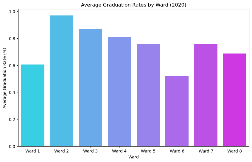
The following bar chart shows the number of discipline incidents reported per ward. To calculate this, I used .sum().
Interpretations: - Ward 5 has the most incidents, with over 800 in counting, a lot compared to other wards - Wards 7 and 1 are also substantially higher, with more than 600 incidents - Wards 2 and 6 have much lower totals - Ward 6 is just nearing 100, which is interesting since it also has lower AP/IB participation. – This may be due to smaller class sizes or smaller schools in general and, therefore, fewer incidents and, unfortunately, fewer resources. - Wards 3, 4, and 8 fall in the middle, with totals ranging between 400 and 500 incidents.
# Group by discipline metric score by ward to get total
discipline_by_ward = discipline_summary.groupby(['ward'], as_index=False)['discipline metric score'].sum().reset_index()

# # sort by discipline total
# discipline_by_ward = discipline_by_ward.sort_values(by='discipline metric score', ascending=False)

# Plotting
plt.figure(figsize=(10,6))
sns.barplot(data=discipline_by_ward, x='ward', y='discipline metric score', palette='cool')

# Customize
plt.title('Total Discipline Incidents By Ward (2020)')
plt.xlabel('Ward')
plt.ylabel('Total Incidents')
plt.show()
/var/folders/ph/mfm_2j1s57n8ylwflpqw64840000gn/T/ipykernel_72077/413252027.py:9: FutureWarning:
Passing `palette` without assigning `hue` is deprecated and will be removed in v0.14.0. Assign the `x` variable to `hue` and set `legend=False` for the same effect.
sns.barplot(data=discipline_by_ward, x='ward', y='discipline metric score', palette='cool')
I calculated the average AP/IB participation metric across the wards using group by.
Interpretations:
- Ward 2 leads again, with almost 100% of students participating in advanced placement courses.
- Wards 6, 7, and 8 have lower participation rates, with 8 at the bottom.
- Wards 3, 4, and 5 are doing pretty well, with participation rates closer to 60-70%
# Group by test metric scores by ward to calculate average AP participation
test_summary = filtered_test.groupby('ward', as_index=False)['test metric score'].mean().reset_index()

# Sort by participation rate
# test_summary = test_summary.sort_values(by='test metric score', ascending=False)

# Plotting
plt.figure(figsize=(10,6))
sns.barplot(data=test_summary, x='ward', y='test metric score', palette='cool')

# Customizing the plot
plt.title('Average AP/IB Participation Rate by Ward (2020)', fontsize=16)
plt.xlabel('Ward', fontsize=12)
plt.ylabel('Average Participation Rate (%)', fontsize=12)
plt.ylim(0, 1)  # Since the metric is a percentage converted to a decimal
plt.tight_layout()

# Show the plot
plt.show()
/var/folders/ph/mfm_2j1s57n8ylwflpqw64840000gn/T/ipykernel_72077/3331951230.py:9: FutureWarning:
Passing `palette` without assigning `hue` is deprecated and will be removed in v0.14.0. Assign the `x` variable to `hue` and set `legend=False` for the same effect.
sns.barplot(data=test_summary, x='ward', y='test metric score', palette='cool')
I used .describe() on the ‘attendance,’ ‘discipline,’ and ‘test’ datasets to get the summary statistics for each:
Attendance Summary:
- Mean: About 86% of students attended school
- Range: Attendance rates vary from a low of 61% to a high of 96%
- Most schools appear to have high attendance, with 75% above 84%, but there are still a few outliers at the lower end
Discipline Summary:
- Mean: Schools reported around 110 discipline incidents
- Range: The number of incidents spans from 9 to 293
- Spread:
- Half the schools report less than 78 incidents
- The top 25% of schools have over 172 incidents - indicating that discipline issues are concentrated in a smaller number of schools
Test Summary:
- Mean: About 53% of students participate in AP/IB programs
- Range: Participation ranges from 5% to 99%
- Spread:
- 50% of schools have participation below 47%
- The top 71% of schools are doing better, with participation rates above 71%.
# Summary statistics for filtered_attendance
attendance_summary = filtered_attendance['attendance metric score'].describe()

# Summary statistics for discipline_summary
discipline_summary_stats = discipline_summary['discipline metric score'].describe()

# Summary statistics for filtered_test
test_summary_stats = filtered_test['test metric score'].describe()

# Display summary statistics
print("Attendance Summary:")
print(attendance_summary)

print("\nDiscipline Summary:")
print(discipline_summary_stats)

print("\nTest Summary:")
print(test_summary_stats)
Attendance Summary:
count 33.000000
mean 0.860909
std 0.097927
min 0.610000
25% 0.840000
50% 0.900000
75% 0.930000
max 0.960000
Name: attendance metric score, dtype: float64
Discipline Summary:
count 33.000000
mean 109.939394
std 85.891989
min 9.000000
25% 47.000000
50% 78.000000
75% 172.000000
max 293.000000
Name: discipline metric score, dtype: float64
Test Summary:
count 30.000000
mean 0.532000
std 0.279672
min 0.050000
25% 0.357500
50% 0.470000
75% 0.715000
max 0.990000
Name: test metric score, dtype: float64In the following cell, I ran another correlation matrix, observing on the ward level. Let’s go over some strong negative and positive correlations and some interesting insights from the correlation matrix.
Strong Positive Correlations:
The Poverty rate and the Black population have a correlation coefficient of about 0.95, which indicates that wards with higher poverty tend to have a higher proportion of the Black population.
We also see that Median Household Income and Grocery Store Count have a correlation coefficient of about 0.93, which indicates that as median household income increases, so does the number of grocery stores in the area.
Strong Negative Correlations:
Poverty Rate and Grocery Store Count have a correlation coefficient of about -0.93, reinforcing our previous observation that there are fewer grocery stores in areas with higher poverty rates.
We also have Attendance Metric Score and Black population, with a correlation coefficient of about -0.80. This indicates a lack of attendance within wards with a higher Black population.
Some Interesting Trends:
Crime Count has weak correlations with most variables, which could be attributed to the fact that crime count can only account for crimes that have been reported and criminals that have been caught. Therefore, we may not be getting its true impact.
Test Metric Score and Poverty Rate have a negative correlation of about -0.61. So, while poverty has a noticeable impact on test scores, it is not necessarily dominant.
One of the more interesting trends is the strong correlation between Attendance Metric Score and socioeconomic indicators, notably Grocery Store Count. We will observe these patterns further with some statistical tests to see if we can reveal any meaningful relationships before we move into machine learning.
correlation_matrix = wardlevel_df.corr()

# Plot heatmap
plt.figure(figsize=(10, 8))
sns.heatmap(correlation_matrix, annot=True, cmap='coolwarm', fmt=".2f")
plt.title("Correlation Heatmap of Indicators")
plt.show()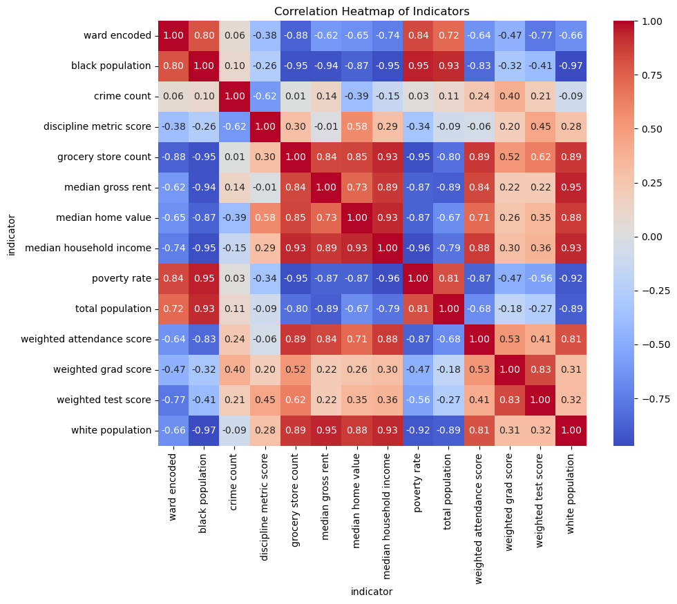
I will start with a Pearson correlation test to assess the strength and significance of our observed correlations. I will use the actual count column we created earlier to calculate the weighted averages of the attendance, test, and graduate data per school by ward.
With a correlation of 0.89 and a P-value of 0.0034, this result confirms that wards with more grocery stores tend to have higher school attendance rates.
# Example: Correlation between poverty rate and weighted attendance score
x = wardlevel_df['grocery store count']
y = wardlevel_df['weighted attendance score']

correlation, p_value = pearsonr(x, y)
print(f"Correlation: {correlation:.2f}, P-value: {p_value:.4f}")
Correlation: 0.89, P-value: 0.0034I decided to transition away from the ward level and look at the data at the school level. Next, I ran a Pearson correlation test to explore the relationship between median household income and graduation rates.
The results are a correlation of 0.37 and a P-value of 0.0566. The correlation is positive and moderate. The P-value is slightly above the 0.05 threshold.
x = refined_df['median household income']
y = refined_df['graduate rate']

correlation, p_value = pearsonr(x, y)
print(f"Correlation: {correlation:.2f}, P-value: {p_value:.4f}")
Correlation: 0.37, P-value: 0.0556I looked at the relationship between grocery store count and attendance metric score again, but this time on the school level.
The correlation came to 0.39, and the P-value came to 0.0430. This lets us know that there is a moderate positive relationship and that it is unlikely that this relationship is due to chance. This reinforces the idea that community resources play a role in student attendance.
x = refined_df['grocery store count']
y = refined_df['attendance metric score']

correlation, p_value = pearsonr(x, y)
print(f"Correlation: {correlation:.2f}, P-value: {p_value:.4f}")
Correlation: 0.39, P-value: 0.0430There seems to be a positive correlation between attendance and median income by ward, with wards such as Ward 2 and Ward 3 having higher attendance and incomes and lower-income wards like Wards 7 and 8 having the lowest attendance rates.
sns.lmplot(data=wardlevel_cat_df, x='weighted attendance score', y='median household income', hue='ward')
plt.title("Attendance vs. Median Income by Ward")
plt.show()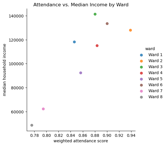
Similarly to attendance, there is a positive trend between AP/IM participation rate and median household income. Again, Wards 2 and 3 showed the highest participation rate, and Wards 7 and 8 showed the lowest.
sns.lmplot(data=wardlevel_cat_df, x='weighted test score', y='median household income', hue='ward')
plt.title("AP/IB Participation vs. Median Income by Ward")
plt.show()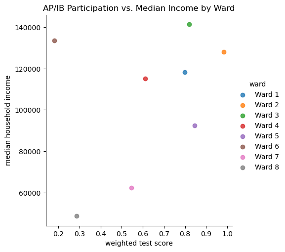
There is a relatively positive relationship between graduation rates and median household income, where higher incomes in Wards 2 and 3 have higher graduation rates, and Ward 8 has the lowest.
sns.lmplot(data=wardlevel_cat_df, x='weighted grad score', y='median household income', hue='ward')
plt.title("Graduation Rate vs. Median Income by Ward")
plt.show()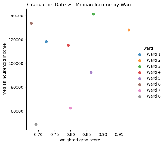
When looking at the relationship between graduation rate and attendance, there is a clear positive trend that a high attendance score results in higher graduation rates for the schools. There is an outlier though, ward 6.
sns.lmplot(data=wardlevel_cat_df, x='weighted grad score', y='weighted attendance score', hue='ward')
plt.title("Graduation Rate vs. Attendance by Ward")
plt.show()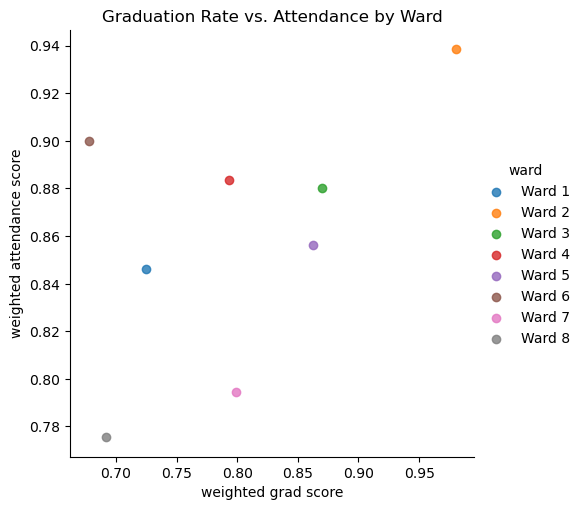
I decided to add a heat map with just some of the highly correlated data, to use in my report to show other how highly correlated the socioeconomic features are with student success indicators.
import pandas as pd
import seaborn as sns
import matplotlib.pyplot as plt

# Subset of Key Variables
key_vars = ['weighted attendance score', 'weighted grad score',
            'grocery store count', 'poverty rate',
            'median household income', 'black population', 'white population']

# Subset the DataFrame to include only the key variables
key_corr = wardlevel_cat_df[key_vars].corr()

# Plot the Focused Heatmap
plt.figure(figsize=(10, 8))
sns.heatmap(key_corr, annot=True, cmap='coolwarm', fmt=".2f", vmin=-1, vmax=1, linewidths=0.5)
plt.title("Correlation Heatmap of Key Indicators")
plt.show()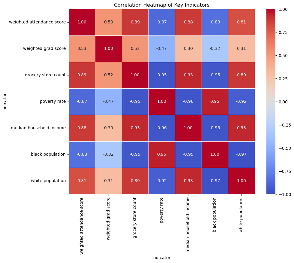
Conclusion
Key Findings
Strong Positive Correlations:
Poverty Rate and Black Population show a high positive correlation (~0.95), meaning wards with higher poverty rates also have a higher proportion of Black residents.
Median Household Income and Grocery Store Count have a positive correlation (~0.93), which suggests that wealthier wards have better access to grocery stores.
Strong Negative Correlations:
Poverty Rate and Grocery Store Count are negatively correlated (~ -0.93) - reinforcing the previous observation that wards suffering from poverty also lack grocery store access.
Attendance Metric Score and Black Population have a negative correlation (- ~0.80), which indicates lower attendance rates in wards with higher Black populations.
Interesting Trends:
Ward 3 maintained a high graduation rate despite high discipline scores, while Ward 8 had substantially fewer discipline incidents and a much lower graduation rate.
Crime Count showed weak correlations with most features, which leads me to wonder if this could indicate underreporting or inconsistencies in the crime data.
Pearson Correlation Tests:
- A positive correlation of 0.39 (P-value 0.043) between Grocery Store Count and Weighted Attendance Score suggests that better grocery access may influence attendance rates.
Issues in the Data:
Missing Values - Some datasets had missing rows or NaN values, particularly the graduation rate and discipline datasets, so I did my best to rectify this - whether that was dropping the rows or filling the values to maintain data quality
Disparities Across Wards - Certain schools and wards consistently underperform, while others show better success metrics which could introduce bias during modeling.
Crime Data - As mentioned before, the weak correlations with crime counts are a cause for concern
Next Steps
Feature Selection and Standardization
I focused on selecting relevant, meaningful features that were not highly correlated with each other to avoid multicollinearity. Features were selected based on their correlation with student success indicators, which was realized through the heatmap for the correlation matrix.
Final Features:
- Student Success Indicators: Weighted Attendance Score, Weighted Test Score, Weighted Graduation Rate
- Socioeconomic Features: Median Household Income and Poverty Rate
- Demographics: Black Population and White Population
- Community: Grocery Store Count
- Ward: Kept for analysis and grouping purposes
Additionally, I standardized all the numeric features using StandardScaler to ensure that all features were scaled consistently, preventing any one feature from dominating the model simply because of its range of values.