import pandas as pd
import numpy as np
import seaborn as sns
import matplotlib.pyplot as plt
from sklearn.preprocessing import OneHotEncoder
from sklearn.preprocessing import LabelEncoder
from sklearn.model_selection import train_test_split
from sklearn.linear_model import LinearRegression
from sklearn.linear_model import LogisticRegression
from sklearn.preprocessing import StandardScaler
from sklearn.metrics import mean_squared_error, accuracy_score
from sklearn.ensemble import BaggingClassifier, BaggingRegressor
from sklearn.decomposition import PCA
from sklearn.manifold import TSNE
from sklearn.model_selection import cross_val_score
from sklearn.tree import DecisionTreeClassifier
from sklearn.metrics import classification_report, confusion_matrix
from sklearn.tree import DecisionTreeRegressor
from sklearn.neighbors import KNeighborsClassifier
from sklearn.ensemble import RandomForestClassifierSupervised Learning
For supervised learning, I decided to explore and predict key school-level metrics. The goal is to build models that will help uncover different patterns and maccurately predictschool performance. I aim to answer the following questions:
- What factors contribute most to graduate rates?
- Can we predict which income group a school belongs to based on its features?
I used models like Linear Regression, Decision Tree Regression, and Classifiers to predict continuous and categorical outcomes. My analysis will not only evaluate model performance due to the same dataset but, it will highlight which features are most impactful to provide actionable insights for educators, policymakers, and stakeholders who aim to improve the schools of D.C.
Code
final_df = pd.read_csv('/Users/anilechoice/Documents/georgetown/5000/project-anilechoice00/data/processed-data/ml_df.csv')
print(final_df.head())

print(final_df.shape)

pca_df = pd.read_csv('/Users/anilechoice/Documents/georgetown/5000/project-anilechoice00/data/processed-data/pca_df.csv')
school name attendance metric score ward \
0 Anacostia High School -2.402762 Ward 8
1 BASIS DC PCS 1.116979 Ward 2
2 Ballou High School -2.402762 Ward 8
3 Capital City PCS - High School 0.614159 Ward 4
4 Cardozo Education Campus -0.793738 Ward 1
test metric score graduate rate discipline metric score \
0 -1.071328 -1.610130 -0.234854
1 1.460674 1.234536 -0.800150
2 -1.211995 -1.610130 -1.238544
3 -0.227328 0.717324 -0.131024
4 -0.332828 -1.437726 1.980187
black population white population median household income poverty rate \
0 1.034757 -0.954451 -1.460012 0.170
1 -1.667535 1.766317 1.128581 0.043
2 1.034757 -0.954451 -1.460012 0.170
3 -0.278019 -0.019895 0.705615 0.091
4 -1.256195 0.975707 0.814029 0.063
grocery store count
0 -1.168424
1 1.068558
2 -1.168424
3 0.509313
4 1.068558
(28, 11)To prepare for supervised learning, I started by encoding the ward columns using custom mapping and lebel encoding.
After much trial and error, I realized I could not include school name or ward as encoded columns in my regression analysis, as it introduced multicollinearity. This redundancy made it difficult for the model to make accurate predictions. Once I dropped these columns, the model was able to focus on the unique features. In this first cell, I have the my ward level data, which includes ward as a categorical variable but is then encoded so it can be used for analysis. From my correlation heatmap that I created on this data during EDA, I was able to see which columns I should drop to avoid collinearity. These columns had high corelation with the ones I left. In order for the model to focus on the unique features, it was best that those were dropped.
# Encode the ward column
ward_mapping = {
    'Ward 1': 1, 'Ward 2': 2, 'Ward 3': 3, 'Ward 4': 4,
    'Ward 5': 5, 'Ward 6': 6, 'Ward 7': 7, 'Ward 8': 8
}
final_df['ward_encoded'] = final_df['ward'].map(ward_mapping)

# Drop columns that are unnecessary
final_df = final_df.drop(['grocery store count', 'school name','discipline metric score'], axis=1)

# Check column alignment
print(final_df.columns)

# Initialize LabelEncoder
label_encoder = LabelEncoder()

# Apply label encoding to the ward column
final_df['ward_encoded'] = label_encoder.fit_transform(final_df['ward'])

# View the mapping of labels to numbers
print(dict(zip(label_encoder.classes_, label_encoder.transform(label_encoder.classes_))))

# Treat ward_encoded as categorical
final_df['ward_encoded'] = final_df['ward_encoded'].astype('category')
Index(['attendance metric score', 'ward', 'test metric score', 'graduate rate',
'black population', 'white population', 'median household income',
'poverty rate', 'ward_encoded'],
dtype='object')
{'Ward 1': np.int64(0), 'Ward 2': np.int64(1), 'Ward 3': np.int64(2), 'Ward 4': np.int64(3), 'Ward 5': np.int64(4), 'Ward 6': np.int64(5), 'Ward 7': np.int64(6), 'Ward 8': np.int64(7)}Regression
I prepared a school-level dataset for regression analysis to predict the graduation rate. I started by encoding the ward column using LabelEncoder and dropping ward and school names.
Next, I defined the features (X) and target variable (y): - Target (y): Graduation rate
I performed a train-test split to train the model, keeping 80% of the data for training and reserving the remaining 20% for testing. This is so that the model can be evaluated on unseen data. After this, I trained a Linear Regression model.
# School-level DataFrame
schoollevel_cat_df = final_df.copy()

# Encode the ward column
label_encoder = LabelEncoder()
schoollevel_cat_df['ward_encoded'] = label_encoder.fit_transform(schoollevel_cat_df['ward'])

# Drop unnecessary columns (e.g., school name)
schoollevel_cat_df = schoollevel_cat_df.drop(columns=['ward', 'school name'], errors='ignore')

# Define features (X) and target (y)
X_linear_school = schoollevel_cat_df.drop(columns='graduate rate')
y_linear_school = schoollevel_cat_df['graduate rate']

# Train-test split
X_train_linear, X_test_linear, y_train_linear, y_test_linear = train_test_split(
    X_linear_school, y_linear_school, test_size=0.4, random_state=5000
)

# Train the Linear Regression model
lr = LinearRegression()
lr.fit(X_train_linear, y_train_linear)
LinearRegression()In a Jupyter environment, please rerun this cell to show the HTML representation or trust the notebook.
On GitHub, the HTML representation is unable to render, please try loading this page with nbviewer.org.
LinearRegression()
I started by looking at the model’s y-intercept and coefficients to see the direction of the line in order to evaluate the linear regression model on the training data,
Next, I predicted the graduation rates using the training data and used a scatter plot to visualize the relationship between the actual and predicted values. The points should align fairly well along a diagonal line to be an accurate model.
The plot does show some alignment, but there are some outliers. This lets us know that the model captures some trends, but there is room for improvement.
# Get intercept and coefficients
c = lr.intercept_
m = lr.coef_
print("Intercept:", c)
print("Coefficients:", m)

# Predict on training data
y_pred_train = lr.predict(X_train_linear)

# Scatter plot for actual vs predicted
plt.scatter(y_train_linear, y_pred_train)
plt.xlabel('Actual Graduate Rate')
plt.ylabel('Predicted Graduate Rate')
plt.title('Actual vs Predicted - Linear Regression (Train Data - School Level)')
plt.show()
Intercept: 2.0094125670574434
Coefficients: [ 3.31489252e-02 7.11518442e-01 -8.95461945e-01 -1.34729722e+00
6.11628512e-02 -4.41145918e+01 5.94097743e-01]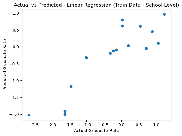
I calculated two key metrics to evaluate the performance of the linear regression model:
Root Mean Square Mean (RMSE): - RMSE measures the model’s prediction error on the training data - an RMSE of 0.496 means that the model’s predictions deviate by about 0.496 from the actual graduation rates - which provides insight into the overall error but needs to tell us how well the model predicts unseen data.
Cross-Validation R Squared Scores: - I performed three-fold cross-validation to assess the model’s ability to generalize. The mean R squared score was 0.2170, better than other tests, such as a four-fold where the mean R squared was negative. Reducing the number of folders might have reduced the variability, which gave more stable results.
These results show that the model could be better, but it still captures some of the data’s relationships.
mse = mean_squared_error(y_train_linear, y_pred_train)
rmse = np.sqrt(mse)
print(f"Root Mean Square Error (RMSE) for Linear Regression: {rmse}")
Root Mean Square Error (RMSE) for Linear Regression: 0.49618817645085816cv_scores = cross_val_score(lr, X_linear_school, y_linear_school, cv=3, scoring='r2')
print(f"Cross-Validation R^2 Scores for Linear Regression: {cv_scores}")
print(f"Mean R^2: {cv_scores.mean():.4f}")Cross-Validation R^2 Scores for Linear Regression: [ 0.41665062 0.31483002 -0.08048596]
Mean R^2: 0.2170I predicted the graduation rates using the test set to evaluate the linear regression model on the unseen data. I measured the performance using R Square, which came to 0.5611. This means the model explains about 56% of the variance in the test set.
When looking at the visualized predictions in the scatter plot, the model captures the data well since the points align along the diagonal for the most part. However, it is important to keep the size of this dataset in mind - since it is small, it can be hard to determine how accurate a model is without a substantially sized set of data to train, validate, and test it.
Overall, the r-squared results and the scatter plot confirm that the model performs moderately well on unseen data, but there is still room for improvement.
# Predict on the test set
y_pred_test = lr.predict(X_test_linear)

# Evaluate performance
test_r2 = lr.score(X_test_linear, y_test_linear)
print(f"Final R Squared on Test Set: {test_r2:.4f}")

# Plot Actual vs Predicted
plt.scatter(y_test_linear, y_pred_test, alpha=0.7)
plt.title('Actual vs Predicted - Linear Regression (Test Set)')
plt.xlabel('Actual')
plt.ylabel('Predicted')
plt.grid(alpha=0.3)
plt.show()
Final R Squared on Test Set: -1.4979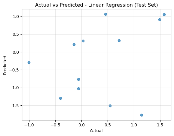
The linear regressor did not perform exceptionally well on my data, so I will run a Decision Tree Regressor to see if a more flexible, nonlinear model improves the performance. I decided to set max_depth to 2 to avoid overfitting.
I extracted the feature importance scores after fitting the model to the training data. These scores highlight which features contribute most to predicting the target variable - in this case, graduation rate. These indicators will help to understand which factors are driving graduation rates.
Finally, I evaluated the model’s performance using Mean Squared Error (MSE), and R squared on the test set to compare it with the linear regression results from earlier.
# Initialize the Decision Tree Regressor
dt_school = DecisionTreeRegressor(max_depth=2, random_state=5000)

# Fit the model on school-level training data
dt_school.fit(X_train_linear, y_train_linear)

# Extract feature importance scores
feature_importances_school = dt_school.feature_importances_

# Predict on test data
y_pred_dt_school = dt_school.predict(X_test_linear)

# Evaluate the model
mse_dt_school = mean_squared_error(y_test_linear, y_pred_dt_school)
r2_dt_school = dt_school.score(X_test_linear, y_test_linear)
The decision tree regressor was evaluated on the test data to predict graduation rates had the following results:
Mean Squared Error: 0.4485 - A moderate reduction in prediction error compared to the linear regression model R squared: 0.2542 - the model explains 25% of the variance in the test data
I also extracted and visualized the feature importance scores: - Attendance was the most significant predictor at 75.6% importance - Ward had an importance of 17.8% - Test scores have an importance of 6.6% - The other features showed zero importance. This suggests that they add little to predicting graduation rates in this model.
The high importance of attendance highlights its strong correlation with graduation rates. Still, the low R-squared suggest there may be some unmodeled complexity or some missing predictive features that could improve the accuracy.
# Print Mean Squared Error & R^2
print(f"Decision Tree MSE Decision Tree Regressor (School Level): {mse_dt_school:.4f}")
print(f"Decision Tree R^2 Decision Tree Regressor (School Level): {r2_dt_school:.4f}\n")

# Create a dataframe for feature importances
importance_df_school = pd.DataFrame({
    'Feature': X_train_linear.columns,
    'Importance': feature_importances_school
}).sort_values(by='Importance', ascending=False)

# Display top features
print(importance_df_school)


# Plot feature importances
plt.figure(figsize=(10, 6))
plt.barh(importance_df_school['Feature'], importance_df_school['Importance'], color='skyblue')
plt.xlabel('Feature Importance')
plt.ylabel('Features')
plt.title('Feature Importance from Decision Tree Regressor (School Level)')
plt.gca().invert_yaxis()  # Invert y-axis for better visualization
plt.grid(axis='x', linestyle='--', alpha=0.7)
plt.show()
Decision Tree MSE Decision Tree Regressor (School Level): 0.7224
Decision Tree R^2 Decision Tree Regressor (School Level): -0.2881
Feature Importance
0 attendance metric score 0.773208
2 black population 0.187557
6 ward_encoded 0.039234
1 test metric score 0.000000
3 white population 0.000000
4 median household income 0.000000
5 poverty rate 0.000000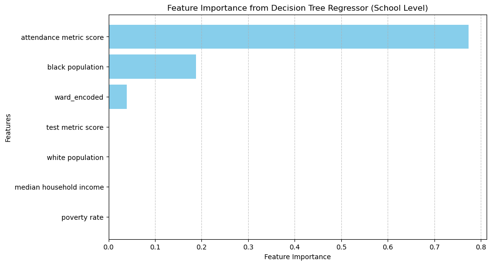
Binary Classification
To predict whether a school has a graduation rate of less than 87%, I prepared the data by redefining the graduation rate:
Schools with a graduation rate of less than 87% were labeled as 1 (low-performing) Schools with a graduation rate above 87% were labeled as 0 (high-performing)
Next, I checked the class balance: - 22 schools were categorized as low-performing - 6 schools were categorized as high-performing
Because of the imbalanced classes, I used a stratified train-test split to ensure both the training and test sets maintained the class proportions. The split used 60% of the data for training and set aside the remaining 40% for testing.
Next, I initialized a decision tree classifier with a max_depth of 3 in order to help balance interpretability with predictive power, and then I trained the model. After training the model, I predicted the test data to evaluate the model’s performance.
# Define features and binary target
X_tree_school = schoollevel_cat_df.drop('graduate rate', axis=1)
y_tree_school = (schoollevel_cat_df['graduate rate'] < 0.87).astype(int)

# Class interpretation:
# 1 -> low performing (graduate rate < 87%)
# 0 -> high performing (graduate rate >=87%)

# Check class balance
print("Class Balance:")
print(y_tree_school.value_counts())

# Split into training and test sets
X_train_tree_school, X_test_tree_school, y_train_tree_school, y_test_tree_school = train_test_split(
    X_tree_school, y_tree_school, test_size=0.4, stratify=y_tree_school, random_state=5000
)

# Initialize Decision Tree Classifier
dtc_school = DecisionTreeClassifier(max_depth=3, random_state=5000)

# Train the model
dtc_school.fit(X_train_tree_school, y_train_tree_school)

# Predict the test data
y_pred_tree_school = dtc_school.predict(X_test_tree_school)
Class Balance:
graduate rate
1 22
0 6
Name: count, dtype: int64I tested the decision tree classifier model’s ability to detect low-performing schools (graduation rate below 87%).
Confusion Matrix: - The model identified two low-performing schools correctly out of 3 - It predicted seven high-performing schools correctly and misclassified 2
I also printed the classification report to better understand the performance.
- 50% of the predicted low-performing schools were accurate
- 88% of the predicted high-performing schools were accurate
The recall for low-performing schools is 67%, which isn’t bad considering the sample size. Finally, the model’s overall accuracy is 75% - decent for a simple decision tree!
To make sure my decision tree wasn’t only performing well on a single train-test split, I ran a 3-fold cross-validation. The accuracy fluctuated slightly, but the model achieved 75% accuracy, which aligns well with the performance on my single test split.
Overall, the step produced a solid model and highlighted some key patterns. There is still room for improvement, but the decision tree provided a great starting point for understanding which factors could drive graduation rates at the school level.
# Confusion Matrix
print('Confusion Matrix:')
cm = confusion_matrix(y_test_tree_school, y_pred_tree_school)
print(cm)

sns.heatmap(cm, annot=True, fmt='d', cmap='Blues', xticklabels=['<=8%', '>8%'], yticklabels=['<=8%', '>8%'])
plt.xlabel('Predicted')
plt.ylabel('Actual')
plt.title('Confusion Matrix (School Level)')
plt.show()

# Classification Report
print('\nClassification Report:')
print(classification_report(y_test_tree_school, y_pred_tree_school, target_names=['<=8%', '>8%']))

# Accuracy
accuracy_school = accuracy_score(y_test_tree_school, y_pred_tree_school)
print(f"Accuracy: {accuracy_school:.4f}")
Confusion Matrix:
[[2 1]
[2 7]]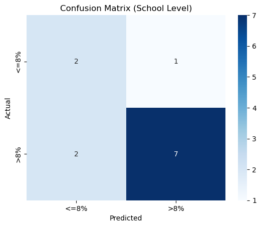
Classification Report:
              precision    recall  f1-score   support

        <=8%       0.50      0.67      0.57         3
         >8%       0.88      0.78      0.82         9

    accuracy                           0.75        12
   macro avg       0.69      0.72      0.70        12
weighted avg       0.78      0.75      0.76        12

Accuracy: 0.7500
# Cross-validation for the Decision Tree Classifier on school-level data
cv_scores_school = cross_val_score(dtc_school, X_tree_school, y_tree_school, cv=3, scoring='accuracy')
print(f"Cross-Validation Accuracy Scores of Decision Tree (School Level): {cv_scores_school}")
print(f"Mean Cross-Validation Accuracy of Decision Tree (School Level): {cv_scores_school.mean():.4f}")Cross-Validation Accuracy Scores of Decision Tree (School Level): [0.7 0.77777778 0.77777778]
Mean Cross-Validation Accuracy of Decision Tree (School Level): 0.7519Next, I extracted the feature importance scores. From the results:
- Attendance contributed 50.7% to the predictions, which makes sense since attendance is linked to student engagement and success
- Poverty rate contributed 27.5%, suggesting that economic factors also play a role in predicting school performance
- White population contributed 21.9%, reflecting demographic trends in graduation rates
The remaining features have zero contribution to this model. This does not mean they are irrelevant; it is just that this model, in particular, didn’t find these features necessary when splitting the data.
On the other hand, the features that were important to the model are strong indicators that there are significant disparities amongst the wards, as the poverty rate and white population are features that clearly separate the more affluent wards from the rest since the affluent wards have higher white populations and the struggling wards have higher poverty rates.
# Feature importance
feature_importances_school = pd.DataFrame({
    'Feature': X_tree_school.columns,
    'Importance': dtc_school.feature_importances_
}).sort_values(by='Importance', ascending=False)

print("\nFeature Importances (School Level):")
print(feature_importances_school)

# Plot feature importances
plt.figure(figsize=(10, 6))
plt.barh(feature_importances_school['Feature'], feature_importances_school['Importance'], color='skyblue')
plt.xlabel('Feature Importance')
plt.title('Feature Importance from Decision Tree (School Level)')
plt.gca().invert_yaxis()  # Reverse the y-axis for better readability
plt.grid(axis='x', linestyle='--', alpha=0.7)
plt.show()
Feature Importances (School Level):
                   Feature  Importance
0  attendance metric score    0.507692
5             poverty rate    0.273504
3         white population    0.218803
1        test metric score    0.000000
2         black population    0.000000
4  median household income    0.000000
6             ward_encoded    0.000000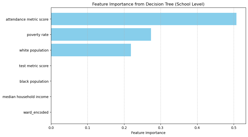
I wanted to see if I could improve the decision tree model’s performance, so I tried a Random Forrest Classifier. Random Forest combines the power of multiple decision trees on random subsets of the data and averaging the predictions. This helps to reduce overfitting and typically has better results than single trees.
I initialized the random forest classifier and trained the model using the same school-level training data. Once I trained the model, the model was able to predict the classes on the test set.
Next, I will evaluate the performance to see if it outperforms the single decision tree.
# Initialize Random Forest Classifier
rf_school = RandomForestClassifier(random_state=5000)

# Train the model on school-level data
rf_school.fit(X_train_tree_school, y_train_tree_school)

# Predict on test data
y_pred_rf_school = rf_school.predict(X_test_tree_school)
Let’s evaluate the model’s performance:
Confusion Matrix:
- The model captured 9 out of 9 high-performing schools
- The model caught 1 out of 3 low-performing schools and misclassified two as high-performing
Classification Report:
- Precision for low-performing schools was 1.00, and this could mean that the model predicting a low-performing school correct every time
- Recall for low-performing schools was 0.33, meaning it only identified 33% of the actual low-performing schools
- For high-performing schools, the precision was 0.82, and the recall was 1.00, which means the model didn’t miss any high-performing school
The overall accuracy was 83.3%, a noticeable improvement from the single decision tree of 75%.
Cross-Validation Results:
I ran a 3-fold cross-validation and got 82.1% for accuracy. This suggests the random forest is more reliable than the single decision tree for this data and target feature.
After getting solid results with the random forest classifier, I tried tuning some hyperparameters to see if I could improve the model’s performance. I tried:
- n_estimator: Increased the number of trees in the forest
- max_depth: Limited the depth of each tree to prevent overfitting
- min_samples_split & sim_samples_leaf: Controlled how the tress split for better predictions
- class_weight: Adjusted for class imbalance to give more weight to the underrepresented group.
These hyperparameters did not improve the model’s performance, suggesting that the random forest is already performing optimally for this data and task. Overall, random forests did well!
# Evaluate the model
print("Confusion Matrix (School Level):")
cm_school = confusion_matrix(y_test_tree_school, y_pred_rf_school)
print(cm_school)

# Visualize Confusion Matrix
sns.heatmap(cm_school, annot=True, fmt='d', cmap='Blues', xticklabels=['<=8%', '>8%'], yticklabels=['<=8%', '>8%'])
plt.xlabel('Predicted')
plt.ylabel('Actual')
plt.title('Confusion Matrix (School Level)')
plt.show()

print("\nClassification Report (School Level):")
print(classification_report(y_test_tree_school, y_pred_rf_school, target_names=['<=8%', '>8%']))

print("\nAccuracy (School Level):", accuracy_score(y_test_tree_school, y_pred_rf_school))
Confusion Matrix (School Level):
[[1 2]
[0 9]]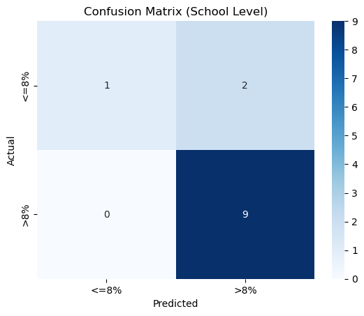
Classification Report (School Level):
              precision    recall  f1-score   support

        <=8%       1.00      0.33      0.50         3
         >8%       0.82      1.00      0.90         9

    accuracy                           0.83        12
   macro avg       0.91      0.67      0.70        12
weighted avg       0.86      0.83      0.80        12


Accuracy (School Level): 0.8333333333333334
# Cross-Validation Scores
cv_scores_school = cross_val_score(rf_school, X_tree_school, y_tree_school, cv=2, scoring='accuracy')
print("Cross-Validation Accuracy Scores of Binary Classifier Random Forest (School Level):", cv_scores_school)
print("Mean Cross-Validation Accuracy of Binary Classifier Random Forest (School Level):", cv_scores_school.mean())Cross-Validation Accuracy Scores of Binary Classifier Random Forest (School Level): [0.85714286 0.78571429]
Mean Cross-Validation Accuracy of Binary Classifier Random Forest (School Level): 0.8214285714285714The feature importance scores from the random forest model show which indicators played the most significant role in predicting graduation rates. Unlike the single decision tree, the random forest distributed importance more evenly across the features.
- Attendance was still the top contributor, with 25.6%, reinforcing its strong connection to graduation rates.
- the second most important contributor was test performance, with 24.6%, which makes sense since test scores often align with academic success.
- The Black population (15.4%) and the White population (10.3%) both carried some weight in the model as well
- Ward, the poverty rate and median household income contributed to the remaining importance of about 8-9%.
The main difference between the decision tree and the random forest is that the random forest gave the Test Metric Score and the demographic indicators much more importance, which balanced out the dominance of a single feature. This highlights the benefit of ensemble methods - they can capture the nuances in the relationships across the data.
The top three contributors, Attendance, Test Metric Score, and Demographics, show that student-level engagement and socioeconomic factors influence the child’s performance and these insights could guide targeted interventions, such as addressing resource gaps in underperforming areas.
# Feature Importances
importances_school = rf_school.feature_importances_
features_school = X_tree_school.columns

# Create a DataFrame for feature importances
feature_importances_school = pd.DataFrame({
    'Feature': features_school,
    'Importance': importances_school
}).sort_values(by='Importance', ascending=False)

print("\nFeature Importances (School Level):")
print(feature_importances_school)

# Plot Feature Importances
plt.figure(figsize=(10, 6))
plt.barh(feature_importances_school['Feature'], feature_importances_school['Importance'], color='skyblue')
plt.xlabel('Feature Importance')
plt.ylabel('Features')
plt.title('Random Forest Feature Importances (School Level)')
plt.gca().invert_yaxis()  # Reverse the y-axis for better readability
plt.grid(axis='x', linestyle='--', alpha=0.7)
plt.show()
Feature Importances (School Level):
                   Feature  Importance
0  attendance metric score    0.256031
1        test metric score    0.246184
2         black population    0.154383
3         white population    0.102725
6             ward_encoded    0.084713
5             poverty rate    0.081451
4  median household income    0.074512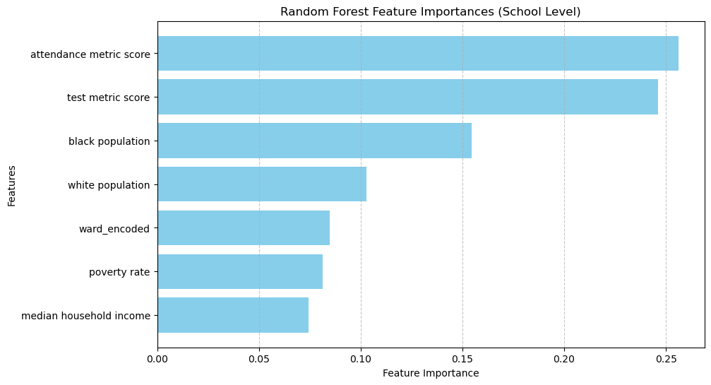
Multi-Class Classification
Now, I am shifting gears into multi-class classification by grouping schools into success tiers based on their composite success metric. This composite metric was calculated by averaging three normalized indicators: graduation rate, attendance metric score, and test metric score. I created the multi-class tiers using pd.qcut, which is a quantile cut. If the dataset were larger, I would have used pd.cut and set the bins to represent specific thresholds for the success metric. However, with the current dataset, pd.qcut worked best, ensuring each group (low, medium, high success) had an even distribution. Once the tiers were created, I followed these steps: Encoded the success tiers (low, medium, high) into numerical labels using LabelEncoder. Defined the socioeconomic features (X) and the multi-class target variable (y). Normalized the features using StandardScaler to ensure that all features were on the same scale, which is critical for distance-based and tree-based models. Performed a train-test split, reserving 20% of the data for testing and stratifying the split to maintain balanced class proportions. I then initialized a Random Forest Classifier using optimal hyperparameters, including a maximum depth of 5, sqrt for feature selection, and a balanced class weight to account for any potential class imbalances. The model was trained on the training data and used to make predictions on the test set. This multi-class grouping introduces a more nuanced classification problem compared to the earlier tasks, as predicting success tiers requires the model to identify complex relationships between socioeconomic factors and the composite success metric. Additionally, Random Forest provides insights into the most influential features driving the classification through feature importance. Next, I will evaluate the performance of the Random Forest model using a confusion matrix, classification report, and feature importance plot.
from sklearn.ensemble import RandomForestClassifier
from sklearn.model_selection import train_test_split
from sklearn.preprocessing import LabelEncoder, StandardScaler

# Define features (X) and target (y)
X_success = schoollevel_cat_df[['poverty rate', 'median household income', 'black population', 'white population', 'ward_encoded']]
y_success = schoollevel_cat_df['success group']

# Encode the target variable (success group)
label_encoder = LabelEncoder()
y_success_encoded = label_encoder.fit_transform(y_success)

# Normalize the features
scaler = StandardScaler()
X_success_scaled = scaler.fit_transform(X_success)

# Train-test split
X_train_success, X_test_success, y_train_success, y_test_success = train_test_split(
    X_success_scaled, y_success_encoded, test_size=0.4, stratify=y_success_encoded, random_state=5000
)


# Initialize and train the Random Forest Classifier
rf_success = RandomForestClassifier(
    random_state=5000,
    n_estimators=100,
    max_depth=5,
    class_weight='balanced',
    max_features ='sqrt',
    min_samples_leaf=1,
    min_samples_split=2
)

# Fit the model on the training data
rf_success.fit(X_train_success, y_train_success)
RandomForestClassifier(class_weight='balanced', max_depth=5, random_state=5000)In a Jupyter environment, please rerun this cell to show the HTML representation or trust the notebook.
On GitHub, the HTML representation is unable to render, please try loading this page with nbviewer.org.
RandomForestClassifier(class_weight='balanced', max_depth=5, random_state=5000)
I evaluated the performance of the Random Forest Classifier for predicting success tiers (low, medium, and high) based on the composite success metric. The key insights from the confusion matrix and classification report are as follows:
Confusion Matrix Insights:
- The high-success group achieved a recall of 50%, meaning two out of four schools in this group were correctly classified.
- The low success group performed with a recall of 75% (three out of four schools correctly classified). Relatively better than the high-success group.
- The medium success group had only one correct prediction out of four samples (25% recall). This highlights that the model struggles to distinguish schools in the medium tier, possibly due to overlapping patterns in socioeconomic features.
Classification Report Summary:
- Precision and F1-scores for the medium success group were notably low - this tells us the model did not perform well in identifying this particular group.
- The overall accuracy on the test set was 50%, suggesting that the model has limited generalization capability for unseen data.
- The macro-average precision, recall, and F1-scores provide a balanced view of the model’s performance but, they remain low due to the inconsistent classification of the medium tier.
Feature Importance Insights:
- The feature importance plot tell us which socioeconomic indicators contributed the most to the model’s predictions:
- White population emerged as the most influential feature, followed by:
- Black population and poverty rate also played significant roles.
- Median household income and ward encoding had moderate contributions, indicating that while income matters, other demographic factors strongly influence the success metric.
- Attendance metric score and graduate rate were less significant for this model.
Key Takeaways:
- The high-success group appears to have more apparent distinguishing patterns, which makes it easier for the model to classify.
- The medium success group remains problematic due to likely overlaps in socioeconomic factors, suggesting that additional features or larger datasets may help refine this classification.
- The Feature importance analysis reveals that demographic factors, particularly population proportions and poverty rate, are strong predictors of school success tiers.
from sklearn.metrics import confusion_matrix, classification_report, accuracy_score
import seaborn as sns
import matplotlib.pyplot as plt

# Predict on the test data
y_pred_rf_success = rf_success.predict(X_test_success)

# Confusion Matrix
cm_rf_success = confusion_matrix(y_test_success, y_pred_rf_success)
print("\nConfusion Matrix (Random Forest - Success Metric):")
print(cm_rf_success)

# Heatmap for Confusion Matrix
plt.figure(figsize=(8, 6))
sns.heatmap(cm_rf_success, annot=True, fmt='d', cmap='Blues', xticklabels=label_encoder.classes_, yticklabels=label_encoder.classes_)
plt.xlabel('Predicted')
plt.ylabel('Actual')
plt.title('Confusion Matrix Heatmap (Random Forest - Success Metric)')
plt.show()

# Classification Report
print("\nClassification Report (Random Forest - Success Metric):")
print(classification_report(y_test_success, y_pred_rf_success, target_names=label_encoder.classes_))

# Accuracy
rf_accuracy = accuracy_score(y_test_success, y_pred_rf_success)
print(f"Random Forest Accuracy: {rf_accuracy:.4f}")
Confusion Matrix (Random Forest - Success Metric):
[[2 0 2]
 [0 3 1]
 [0 3 1]]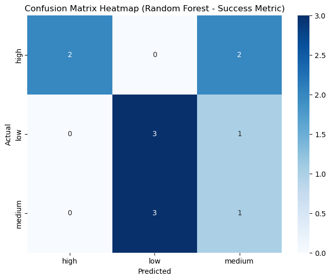
Classification Report (Random Forest - Success Metric):
              precision    recall  f1-score   support

        high       1.00      0.50      0.67         4
         low       0.50      0.75      0.60         4
      medium       0.25      0.25      0.25         4

    accuracy                           0.50        12
   macro avg       0.58      0.50      0.51        12
weighted avg       0.58      0.50      0.51        12

Random Forest Accuracy: 0.5000
# Feature Importance
feature_importances = pd.DataFrame({
'Feature': X_success.columns,
'Importance': rf_success.feature_importances_
}).sort_values(by='Importance', ascending=False)
# Display feature importance
print("\nFeature Importances (Random Forest - Success Metric):")
print(feature_importances)
# Plot feature importance
plt.figure(figsize=(10, 6))
plt.barh(feature_importances['Feature'], feature_importances['Importance'], color='skyblue')
plt.xlabel('Feature Importance')
plt.title('Feature Importance for Random Forest (Success Metric)')
plt.gca().invert_yaxis() # Reverse y-axis for better readability
plt.grid(axis='x', linestyle='--', alpha=0.7)
plt.show()
Feature Importances (Random Forest - Success Metric):
                   Feature  Importance
3         white population    0.275298
2         black population    0.221150
0             poverty rate    0.195554
1  median household income    0.171210
4             ward_encoded    0.136788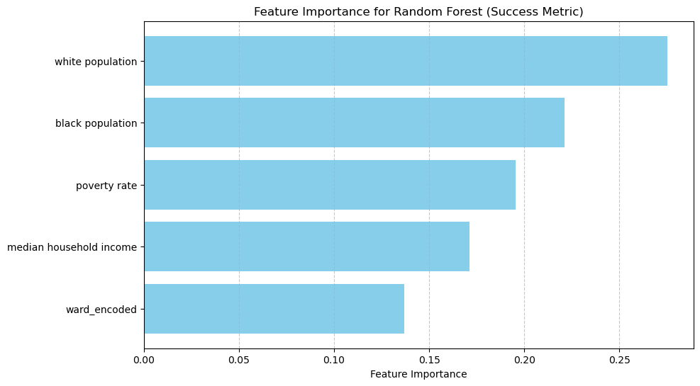
Summary
Challenges
The main difficulty with this data is its size. Unfortunately, small datasets are not well suited for machine learning algorithms as less data means small training, validation, and testing group sizes. Large datasets typically result in a better trained model, therefore resulting in more accurate predictions.
The collinearity of the data, as well as the sample being so small was pretty limiting in regards to statistical testing as well so, I mostly stuck to visualizing the the data and the relationships between different features
A study on individual students and their families suchas sentiment analysis through surveys, asking questions concerning student-teacher relationship,s to food insecurity could expand the analysis of DC public school tremendously. This could provide more insights into student’s lives both inside and outside the class
Benchmarks
- What I discovered in my analysis is, for the most part, what I expected. It aligns with the discourse surrounding the topic of gentrification and its impacts on the residents of the community. From what I learned through my analysis and personal research, D.C. residents has been enduring gentrification since the early 2000s and it is continually progressing. My findings, as well as others, shows that there is a clear correlation between the ward the school belongs to and student performance. There must be an equitable allocation of resources in order to get the schools with Wards 7 and 8 specifically, performing at the level of the other schools.
Conclusion and Future Steps
Based on my analysis, there is evident disparities between schools of the different wards. Higher income areas typically have high student success rates. However, a couple wards were observed to have a higher income median but still showing subpar student success metric. An example of this is Ward 6 - with a median houshold income of $133,590 and a graduation rate below 70%.
Reevaluating the variables for analysis for future studies could prove useful. Many of my variables showed some collinearity, which required me to drop some. A dataset more robust data set - maybe even expanding my scope to middle schools and elementary schools in DC or even to surrounding areas and observing the DMV area as a whole.
Since I used data from peak COVID-19 time, I think that is something to keep in mind when looking at this data, as it is highly possible that this implication had major effects on the indicators I selected for both student success and the social and economic features. To observe possible effects, I think using time series analysis to make connections between pre- COVID-19, in the midsts of it, and then post-COVID-19.
References
Abhishek, R., & Balamurugan, J. (2024, March 28). Impact of social factors responsible for juvenile delinquency - A literature review. Journal of education and health promotion. https://pmc.ncbi.nlm.nih.gov/articles/PMC11081445/
Altaher, N. (2023, March). The Structural Determinants of Health: How Systemic Racism Facilitates Community Violence in D.C. Providence College Digital Commons. https://digitalcommons.providence.edu/health_policy_students/16/?utm_source=digitalcommons.providence.edu%2Fhealth_policy_students%2F16&utm_medium=PDF&utm_campaign=PDFCoverPages
Ashat, D., Tepper, N., & Pawlow, C. (n.d.). An evaluation of food insecurity in the D.C. community. Georgetown Scientific Research Journal. https://gsrjournal.org/index.php/home/article/view/49
Ashtiani, M., & Feliciano, C. (2012). Mentorship and the Postsecondary Educational Attainment of Low-Income Youth. Pathways to Postsecondary Success, 1–6. Baratz, J. C. (n.d.). A Quest for equal education opportunity in a major urban school district: The case of Washington, D.C.; [and] a critique of “a quest for equal educational opportunity in a major urban school district: The case of Washington, D.C.” Policy Commons. https://policycommons.net/artifacts/15418195/a-quest-for-equal-education-opportunity-in-a-major-urban-school-district/16311879/
Butler, A., & Quarles, B. (2024). “it’s a chance, not a choice”: Black families, school choice, and gentrification in Washington, D.C. Teachers College Record: The Voice of Scholarship in Education, 126(2), 120–146. https://doi.org/10.1177/01614681241242878
Freedman’s Bank Building. U.S. Department of the Treasury. (2020, June 1). https://home.treasury.gov/about/history/freedmans-bank-building
Glazerman, S., & Dotter, D. (n.d.). Market signals: How do DC parents rank schools, and what does it mean for policy? policy brief. Policy Commons. https://policycommons.net/artifacts/14755437/market-signals/15655413/
The history and evolution of Anacostia’s Barry Farm. D.C. Policy Center. (2022, January 18). https://www.dcpolicycenter.org/publications/barry-farm-anacostia-history/
Jenkins, D. A. (2020). School reputation as a site of struggle: An investigation of the impact of school choice in Washington, DC on a neighborhood public school. The Urban Review, 52(5), 904–923. https://doi.org/10.1007/s11256-020-00562-2
King, C. J., Buckley, B. O., Maheshwari, R., & Griffith, D. M. (2022). Race, place, and structural racism: A review of health and history in Washington, D.C. Health Affairs, 41(2), 273–280. https://doi.org/10.1377/hlthaff.2021.01805
Logwood, D. C. (2023, November 30). Critical black feminist mentoring: A framework for making black girls’ lives matter. Afterschool Matters. https://eric.ed.gov/?id=EJ1437828
Mann, B., Bennett, H., & Rogers, A. (n.d.). Gentrification, Charter Schools, and Enrollment Patterns in Washington, DC: Shared Growth or New Forms of Educational Inequality?. Taylor & Francis. https://www.tandfonline.com/doi/abs/10.1080/0161956X.2020.1776070
Marinelli, J. A. D. (n.d.). “Education Under Armed Guard”: An Analysis of the School-to-Prison Pipeline in Washington, D.C. Georgetown Law. https://www.law.georgetown.edu/american-criminal-law-review/in-print/volume-59-number-4-fall-2022/education-under-armed-guard-an-analysis-of-the-school-to-prison-pipeline-in-washington-d-c/
McGrath, K. F., & Van Bergen, P. (2015). Who, when, why and to what end? students at risk of negative student–teacher relationships and their outcomes. Educational Research Review, 14, 1–17. https://doi.org/10.1016/j.edurev.2014.12.001
Peiffer, E., Newman, R., Shakesprere, J., Hakizimana, N., & Farrell, L. (2022, August 4). Why community-based facilitators are crucial to the success of Youth Programs. Urban Institute. https://www.urban.org/stories/why-community-based-facilitators-are-crucial-success-youth-programs
Robertson, J. S., Smith, R. W., & Rinka, J. (n.d.). How Did Successful High Schools Improve Their Graduation Rates?. Institute of Educational Science. https://eric.ed.gov/?id=EJ1104424
Shinault, C. M., & Seltzer, R. (2019). Whose turf, whose town? race, status, and attitudes of Washington DC residents toward gentrification. Journal of African American Studies, 23(1–2), 72–91. https://doi.org/10.1007/s12111-019-09427-9
Sullivan, M. D., Campbell, D. B., & Kisida, B. (2008, April). The Muzzled Dog That Didn’t Bark: Charters and the Behavioral Response of D.C. Public Schools. Institute of Education Sciences. https://eric.ed.gov/?id=ED508627
This D.C. tutor-matching organization can’t Find enough volunteers. DCist. (2018, August 24). https://dcist.com/story/18/08/24/dc-tutoring-and-mentoring-initiative/