import pandas as pd
import numpy as np
import os
from sklearn.preprocessing import StandardScaler
from sklearn.decomposition import PCA
import matplotlib.pyplot as plt
from sklearn.manifold import TSNE
from sklearn.cluster import KMeans
from sklearn.metrics import silhouette_score
from sklearn.cluster import DBSCAN
from scipy.cluster.hierarchy import dendrogram, linkage
from scipy.cluster.hierarchy import fcluster
from sklearn.preprocessing import LabelEncoder
import plotly.express as px
from scipy.cluster.hierarchy import dendrogram, linkage
from sklearn.cluster import AgglomerativeClustering

processed_data_path = '/Users/anilechoice/Documents/georgetown/5000/project-anilechoice00/data/processed-data/'Unsupervised Learning
I will perform unsupervised learning algorithms on my data in the following few cells. These include K-Mean, DBSCAN, Hierarchical Clustering, and Principal Component Analysis. Unsupervised learning helps identify patterns and relationships with raw, unlabeled data. This helps to reveal any hidden patterns, trends, or groupings within the data, which can be helpful in further analysis and decision-making.
Code
To prepare the data for unsupervised learning, I began loading in final_df. I needed to one-hot encode the ward columns since unsupervised learning models require numeric inputs. This converts each ward into its binary feature.
Next, I dropped the categorical columns of ‘ward’ and ‘school name’ to ensure only the numeric data remained. Then, I combined the one-hot encoded columns with the rest of the numeric features using pd.concat(). This gave me an entirely numeric dataset ready for machine learning algorithms.
final_df = pd.read_csv('/Users/anilechoice/Documents/georgetown/5000/project-anilechoice00/data/processed-data/ml_df.csv')
# print(final_df.head())

# One hot encode ward
one_hot_ward = pd.get_dummies(final_df['ward'])
# print(one_hot_ward)

without_categorical = final_df.drop(columns=['ward'])
without_categorical = without_categorical.drop(columns=['school name'])

numeric_df = pd.concat([without_categorical, one_hot_ward], axis=1)

# print(numeric_df.head())
print(numeric_df.head())
attendance metric score test metric score graduate rate \
0 -2.402762 -1.071328 -1.610130
1 1.116979 1.460674 1.234536
2 -2.402762 -1.211995 -1.610130
3 0.614159 -0.227328 0.717324
4 -0.793738 -0.332828 -1.437726
discipline metric score black population white population \
0 -0.234854 1.034757 -0.954451
1 -0.800150 -1.667535 1.766317
2 -1.238544 1.034757 -0.954451
3 -0.131024 -0.278019 -0.019895
4 1.980187 -1.256195 0.975707
median household income poverty rate grocery store count Ward 1 Ward 2 \
0 -1.460012 0.170 -1.168424 False False
1 1.128581 0.043 1.068558 False True
2 -1.460012 0.170 -1.168424 False False
3 0.705615 0.091 0.509313 False False
4 0.814029 0.063 1.068558 True False
Ward 3 Ward 4 Ward 5 Ward 6 Ward 7 Ward 8
0 False False False False False True
1 False False False False False False
2 False False False False False True
3 False True False False False False
4 False False False False False False To explore dimensionality reduction and variance structure in the dataset, I applied Principal Component Analysis (PCA). This technique helps to identify the principal components (or directions) that capture the most variance in the data.
The following table summarizes the variance explained by each principal component after applying principal component analysis to the dataset. For principal component 1, 54.95% of the variance in the data is accounted for, and for the first and second principal components, 81.94% of the variance is accounted for. At principal component 8, 98.23% of the data’s variance is accounted for.
These findings will guide the selection of components for further analysis.
# Apply PCA
pca = PCA()
pca_result = pca.fit_transform(numeric_df)

# Explained variance
explained_variance_ratio = pca.explained_variance_ratio_
cumulative_variance = explained_variance_ratio.cumsum()

# Create a DataFrame for explained variance
explained_variance_df = pd.DataFrame({
    'Component': range(1, len(explained_variance_ratio) + 1),
    'Explained Variance': explained_variance_ratio,
    'Cumulative Variance': cumulative_variance
})

print(explained_variance_df)
Component Explained Variance Cumulative Variance
0 1 5.297716e-01 0.529772
1 2 1.644903e-01 0.694262
2 3 1.213647e-01 0.815627
3 4 4.835538e-02 0.863982
4 5 4.349797e-02 0.907480
5 6 3.483040e-02 0.942310
6 7 2.646952e-02 0.968780
7 8 1.279883e-02 0.981579
8 9 1.112003e-02 0.992699
9 10 4.119358e-03 0.996818
10 11 3.181887e-03 1.000000
11 12 2.850139e-33 1.000000
12 13 6.724534e-34 1.000000
13 14 5.306516e-34 1.000000
14 15 2.515206e-34 1.000000
15 16 1.451980e-34 1.000000
16 17 7.440235e-35 1.000000I used an elbow plot to visualize the cumulative explained variance to determine the optimal number of principal components. Although principal component 8 accounts for 98% of the variance, the plot showed me that the explained variance starts to level off at principal component 6. This elbow point indicates that adding more components beyond six does not contribute much-added value.
# Plot cumulative explained variance
plt.plot(range(1, len(cumulative_variance) + 1), cumulative_variance, marker='o')
plt.title('Explained Variance by PCA Components')
plt.xlabel('Number of Components')
plt.ylabel('Cumulative Explained Variance')
plt.grid()
plt.show()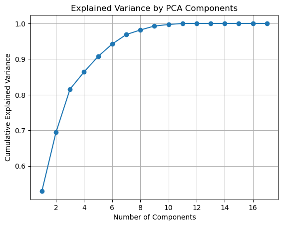
Next, I performed dimensionality reduction by selecting the optimal number of principal components, which I discovered in the first step to be 6. I initialized Principal Component Analysis to use on the data. Once I fit the PCA model to the data, it will be in the reduced-dimensional space, with just the six components. We are left with ‘pca_result_optimal’ as the new dataset with the same rows but only six columns as the principal components.
The print statement shows us that with six components, 98% of the variance is accounted for, meaning the majority of the information in the original data is preserved while reducing its complexity.
# Select the optimal number of components
optimal_components = 6
pca_optimal = PCA(n_components=optimal_components)
pca_result_optimal = pca_optimal.fit_transform(numeric_df)

# Print explained variance of the selected components
print(f"Explained variance by {optimal_components} components: {pca_optimal.explained_variance_ratio_.sum():.2f}")
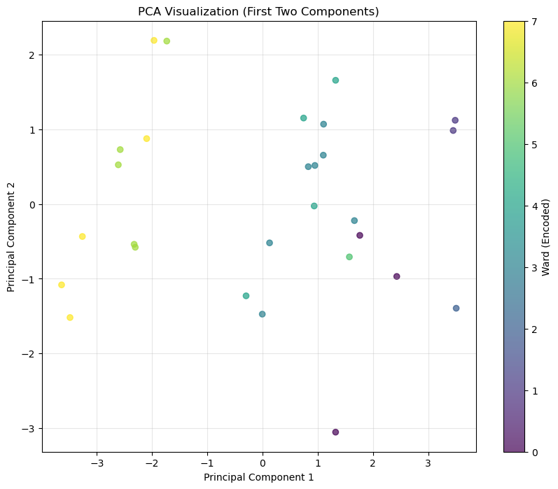
Explained variance by 6 components: 0.94To visualize the results of the PCA, I pulled the first two principal components from the reduced dataset. I created a scatter plot where each point represents a school, and the first two components determine the position. I also encoded the ward variable numerically and used it to color the points in the plot to highlight the patterns across wards.
This visualization helps to explore the distribution of schools in the reduced-dimensional space and identify any patterns or clusters for the wards.
# Extract the first two principal components
pca_df = pd.DataFrame(pca_result_optimal, columns=[f'PC{i+1}' for i in range(pca_result_optimal.shape[1])])
pca_df['ward'] = final_df['ward']  # Using ward for color coding

# Encode ward as numeric
label_encoder = LabelEncoder()
pca_df['ward_encoded'] = label_encoder.fit_transform(final_df['ward'])

# Plot the first two principal components
plt.figure(figsize=(10, 8))
scatter = plt.scatter(pca_df['PC1'], pca_df['PC2'], c=pca_df['ward_encoded'], alpha=0.7)
plt.colorbar(scatter, label='Ward')
plt.title('PCA Visualization (First Two Components)')
plt.xlabel('Principal Component 1')
plt.ylabel('Principal Component 2')
plt.grid(alpha=0.3)
plt.show()
I was curious about a 3D plot since two components only capture a little of the variance in my data. Each axis represents one of the components (PC1, PC2, PC3), and the points are color-coded by ward so that we can better identify the patterns and relationships.
Including the third principal component allows us to uncover additional variance and structure that wasn’t visible in the 2D plot, providing a better understanding of the distribution of schools.
# Create a DataFrame for the first three principal components
pca_3d_df = pd.DataFrame(pca_result[:, :3], columns=['PC1', 'PC2', 'PC3'])
pca_3d_df['ward'] = final_df['ward']  # Add the ward column for color coding

# Create the 3D scatter plot
fig = px.scatter_3d(
    pca_3d_df,
    x='PC1',
    y='PC2',
    z='PC3',
    color='ward',  # Color by ward
    title='3D PCA Visualization (First Three Components)',
    labels={'PC1': 'Principal Component 1', 'PC2': 'Principal Component 2', 'PC3': 'Principal Component 3'},
    opacity=0.7
)

# Customize layout
fig.update_layout(
    scene=dict(
        xaxis_title='PC 1',
        yaxis_title='PC 2',
        zaxis_title='PC 3'
    ),
    coloraxis_colorbar=dict(title='Ward'),
)

# Show the plot
fig.show()
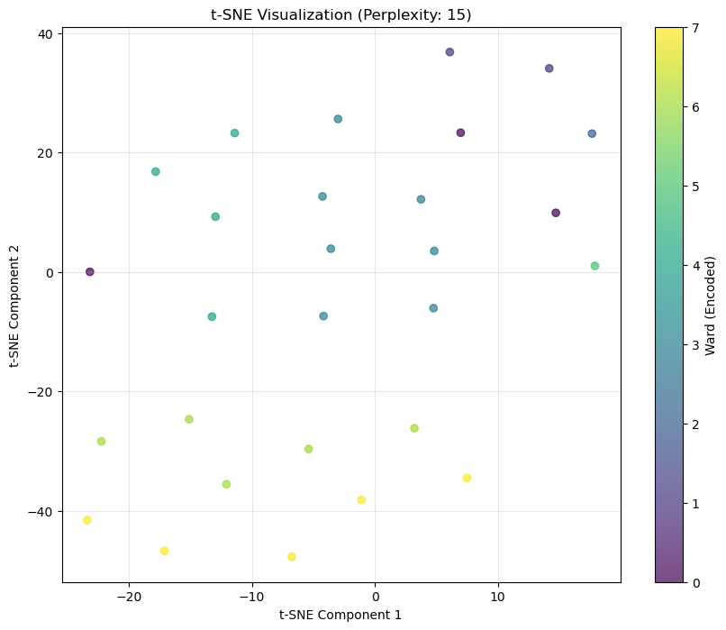
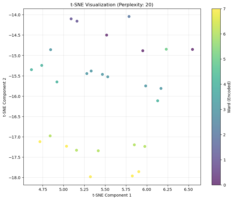
Unable to display output for mime type(s): application/vnd.plotly.v1+jsonNext, I applied t-Distribution Stochastic Neighbor Embedding (t-SNE), a non-linear dimensionality reduction technique that helps visualize high-dimensional data in 2D. I started by encoding the ward column numerically to color-code the pattern across wards.
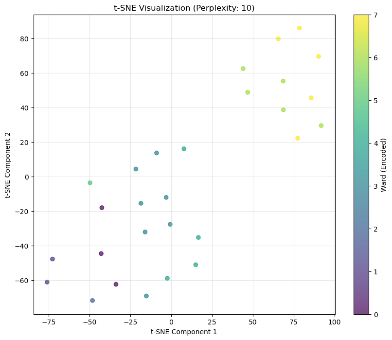
I plotted with different perplexity values (5, 10, 15, 20) to compare how the visualization changes. Perplexity controls the balance between local and global relationships in the data, where lower values focus on local patterns and higher values focus on the broader structure.
Each plot shows the distribution of schools in the reduced space, with the points colored by ward.
# Encode ward
ward_encoded = label_encoder.fit_transform(final_df['ward'])

# Loop over the various perplexities and create a tsne plot for each
for perplexity in [5, 10, 15, 20]:
    tsne = TSNE(n_components=2, perplexity=perplexity, random_state=5000)
    tsne_result = tsne.fit_transform(numeric_df)

    # Convert to DataFrame
    tsne_df = pd.DataFrame(tsne_result, columns=['TSNE1', 'TSNE2'])
    tsne_df['ward_encoded'] = ward_encoded

    # Visualize
    plt.figure(figsize=(10, 8))
    scatter = plt.scatter(tsne_df['TSNE1'], tsne_df['TSNE2'], c=tsne_df['ward_encoded'], alpha=0.7)
    plt.colorbar(scatter, label='Ward')
    plt.title(f't-SNE Visualization (Perplexity: {perplexity})')
    plt.xlabel('t-SNE Component 1')
    plt.ylabel('t-SNE Component 2')
    plt.grid(alpha=0.3)
    plt.show()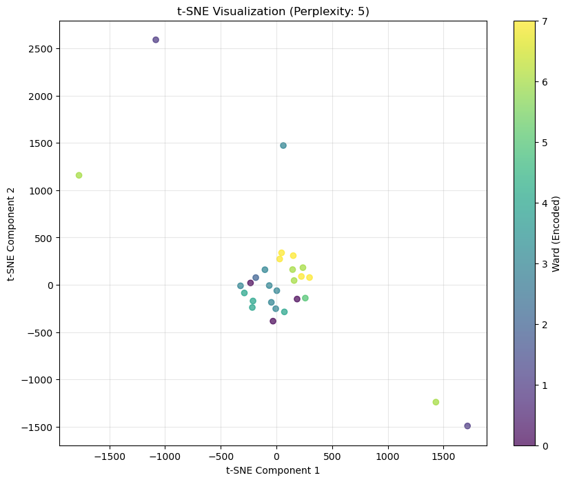
To identify any clusters in the data, I applied K-Means clustering with 8 clusters since I know there are eight wards. K-Means groups data points into clusters based on their distance from cluster centroids.
After fitting the model, I added the cluster labels to the dataset for visualization. I also calculated the Silhouette Score to determine the clustering performance, which reached 0.448. This suggests that the data exhibits some meaningful structure, but this score is not the most substantial.
Finally, I visualized the clusters on the t-SNE plot, using color to distinguish between the clusters or wards.
from sklearn.cluster import KMeans
from sklearn.metrics import silhouette_score
import matplotlib.pyplot as plt

# Apply K-Means
kmeans = KMeans(n_clusters=8, random_state=42)
kmeans_labels = kmeans.fit_predict(tsne_df[['TSNE1', 'TSNE2']])

# Add k-means labels to the t-sne dataset for visualization
numeric_df['KMeans_Cluster'] = kmeans_labels

# Evaluate Silhouette Score
kmeans_silhouette = silhouette_score(numeric_df, kmeans_labels)
print(f"Silhouette Score for K-Means: {kmeans_silhouette}")

# Visualize K-Means Clusters
plt.figure(figsize=(10, 8))
plt.scatter(tsne_df['TSNE1'], tsne_df['TSNE2'], c=kmeans_labels, alpha=0.7)
plt.colorbar(label='Ward')
plt.title('t-SNE Visualization with K-Means Clusters')
plt.xlabel('t-SNE Component 1')
plt.ylabel('t-SNE Component 2')
plt.grid(alpha=0.3)
plt.show()
Silhouette Score for K-Means: 0.5027822343485535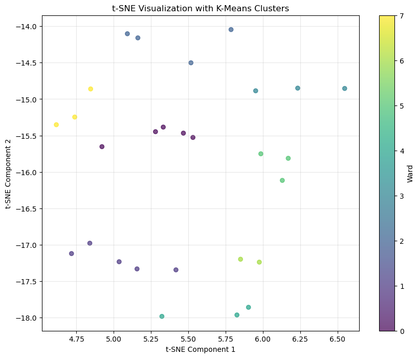
For my following clustering algorithm, I applied DBSCAN (Density-Based Spatial Clustering of Applications with Noise) to the t-SNE results. DBSCAN groups points based on their density, making it effective for clustering points of different shapes and sizes while also accounting for noise.
After fitting the model, I added the DBSCAN labels to the dataset. Then, I calculated the Silhouette score to determine the performance, which gave me a score of 0.778. This tells me that DBSCAN identified more meaningful clusters than K-Means.
Finally, I again visualized the DBSCAN groupings on the t-SNE plot using color coding for the wards.
from sklearn.cluster import DBSCAN

# Apply DBSCAN
dbscan = DBSCAN(eps=0.3, min_samples=3)
dbscan_labels = dbscan.fit_predict(tsne_df[['TSNE1', 'TSNE2']])

# Add labels to the dataset for visualization
numeric_df['DBSCAN_Cluster'] = dbscan_labels

# Evaluate Silhouette Score
valid_points = dbscan_labels != -1
if valid_points.sum() > 1:  # Check if there are enough points to compute
    dbscan_silhouette = silhouette_score(numeric_df[valid_points], dbscan_labels[valid_points])
    print(f"Silhouette Score for DBSCAN: {dbscan_silhouette}")
else:
    print("Not enough valid clusters for silhouette analysis.")

# Visualize DBSCAN Clusters
plt.figure(figsize=(10, 8))
plt.scatter(tsne_df['TSNE1'], tsne_df['TSNE2'], c=ward_encoded, alpha=0.7)
plt.colorbar(label='Ward')
plt.title('t-SNE Visualization with DBSCAN Clusters')
plt.xlabel('t-SNE Component 1')
plt.ylabel('t-SNE Component 2')
plt.grid(alpha=0.3)
plt.show()
Silhouette Score for DBSCAN: 0.7775477410732464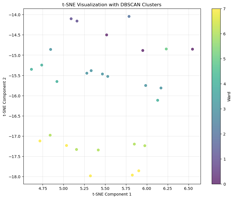
Next, I performed hierarchical clustering using Ward’s method, which helps minimize variance instead of measuring distance. I did this because I knew from the EDA that certain schools didn’t group well with their respective wards.
Next, I applied Agglomerative Clustering using 8 clusters to the t-SNE results. Agglomerative clustering is a bottom-up approach where all points start as their cluster and merge from there. I visualized the resulting clusters on the t-SNE plot, color-coding the points by their hierarchical cluster assignments.
# Perform hierarchical clustering
linkage_matrix = linkage(numeric_df, method='ward')

# Plot Dendrogram
plt.figure(figsize=(10, 8))
dendrogram(linkage_matrix)
plt.title('Hierarchical Clustering Dendrogram')
plt.xlabel('Samples')
plt.ylabel('Distance')
plt.show()

# Apply agglomerative clustering on tsne
agg_clustering = AgglomerativeClustering(n_clusters=8)
agg_labels = agg_clustering.fit_predict(tsne_df[['TSNE1', 'TSNE2']])

# Add labels to the dataset for visualization
numeric_df['Hierarchical_Cluster'] = agg_labels

# Silhouette score
hierarchical_silhouette = silhouette_score(numeric_df, agg_labels)
print(f"Silhouette Score for Hierarchical Clustering: {hierarchical_silhouette:.3f}")

# Visualize Hierarchical Clusters
plt.figure(figsize=(10, 8))
plt.scatter(tsne_df['TSNE1'], tsne_df['TSNE2'], c=ward_encoded, alpha=0.7)
plt.colorbar(label='Hierarchical Cluster')
plt.title('t-SNE Visualization with Hierarchical Clusters')
plt.xlabel('t-SNE Component 1')
plt.ylabel('t-SNE Component 2')
plt.grid(alpha=0.3)
plt.show()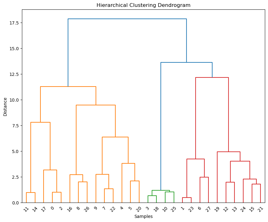
Silhouette Score for Hierarchical Clustering: 0.479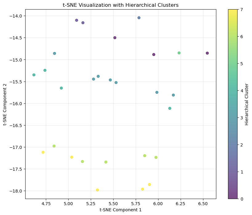
Next, I saved the dimensionality reduction data to my processed data folder.
pca_file_path = processed_data_path + 'pca_df.csv'
pca_df.to_csv(pca_file_path, index=False)
Clustering Methods
K-Means Clustering
K-Means is a clustering method that splits the data into a set number of clusters (in my case, 8). It does this by:
- Assigning points to the nearest cluster center or centroid
- Recalculating the cluster center based on the average of the points in each cluster
- This repeats until there is no change in the clustering
To determine how well the clusters fit the data, I used the Silhouette Score. This tell us how well a point fits into its cluster compared to others. With a score of 0.448, this isn’t the best so, that tells us there was some structure but K-Means didn’t capture the full complexity of the data.
DBSCAN Clustering
I also applied DBSCAN, a density-based method that doesn’t require me to input the number of clusters. Instead, it looks for dense regions and separates them from sparse regions. I used parameters esp=0.3, which is the radius for neighborhood size, and min_samples=3, which is the minimum point to form a cluster. I also tried 1 for min sample, but it had a much lower Silhouette Score - even though there is a ward with only one school (ward 3). This probably means that even though it may be of a different ward, it still shares some similarities with schools of the other wards.
Something interesting about DBSCAN is that it identifies outliers intuitively, marking points that dont belongin any cluster. The Silhouette Score for DBSCAN was 0.778, which is a big improvement from K-Means. This lets us know that the DBSCAN method found more meaningful clusters compared to K-Means.
Hierarchical Clustering
Lastly, I performed Hierarchical Clustering using Ward’s method in order to to keep the variance low. I visualized the results with a dendrogram to show how the clusters form and merge as the distance increases.
Then, I applied agglomerative clustering (a form of hierarchical clustering) to the t-SNE results, again specifying 8 clusters. It did provide a clear breakdown of relationships, but the Silhouette Score was 0.479. So, the clusters weren’t as precise as the DBSCAN. The dendrogram did give a great overall view of the data’s connection, though.
Results
K-Means Results
I produced 8 clusters with K-Mean,, which I plotted the the t-SNE visualization. The clusters were clear but a 0.448 Silhouette Score tell us that there weren’t tight or well-seperated. There wasn’t a strong alignment between the clusters to the ward grouping so K-Means may not handle the more complex relationships in this data well.
DCSCAN Results
DBSCAN performed much better than K-Means. It found clusters that made more sense to the data, achieving a Silhouette Score of 0.778. DBSCAN was able to capture the underlying structure since the clusters on the t-SNE plot aligned better with the ward labels.
Hierarchical Clustering Results
The dendrogram from hierarchical clustering showed clear breakdowns in grouping, which is useful for understanding how groups merge at different levels. When I applied agglomerative clustering with 8 clusters to the t-SNE results, the clustering was not as good as the clustering I saw with DBSCAN. However, this method was still useful for seeing how the schools relate to each other.
Conclusion
- DBSCAN performed the best with tighter clusters and a higher Silhouette score
- K-Means struggled to capture the complexities of the data, but it still provided an understanding of the partitioning of the data
- Hierarchical clustering was useful for visualizing relationships