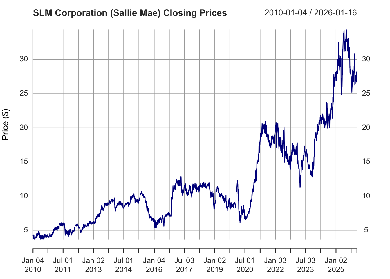
For this analysis, we examine the stock returns of SLM Corporation (Sallie Mae), one of the largest student loan servicers in the United States. Given the central theme of this project—the intersection of student loan debt and housing markets—analyzing Sallie Mae’s stock volatility provides unique insights into market perceptions of the student lending industry.
Sallie Mae’s stock returns are subject to volatility clustering, a phenomenon where periods of high volatility tend to cluster together. This makes it an ideal candidate for ARCH/GARCH modeling, which specifically captures time-varying volatility in financial returns.
Data Preparation
Show Code
# Fetch SLM stock data from Yahoo Finance# Using data from 2010 to present for sufficient observationsgetSymbols("SLM", from ="2010-01-01", to =Sys.Date(), src ="yahoo")
[1] "SLM"
Show Code
# Calculate log returns (more appropriate for financial modeling)slm_returns <-na.omit(diff(log(Cl(SLM))))colnames(slm_returns) <-"returns"# Convert to numeric vector for modelingreturns_vec <-as.numeric(slm_returns)returns_ts <-ts(returns_vec)# Display summary statisticscat("Summary Statistics for SLM Daily Log Returns:\n")
Summary Statistics for SLM Daily Log Returns:
Show Code
summary(returns_vec)
      Min.    1st Qu.     Median       Mean    3rd Qu.       Max.
-0.1959737 -0.0099758  0.0006272  0.0004644  0.0113536  0.2555788
# Plot the stock priceplot(Cl(SLM), main ="SLM Corporation (Sallie Mae) Closing Prices",ylab ="Price ($)", col ="darkblue", lwd =1.5)
Show Code
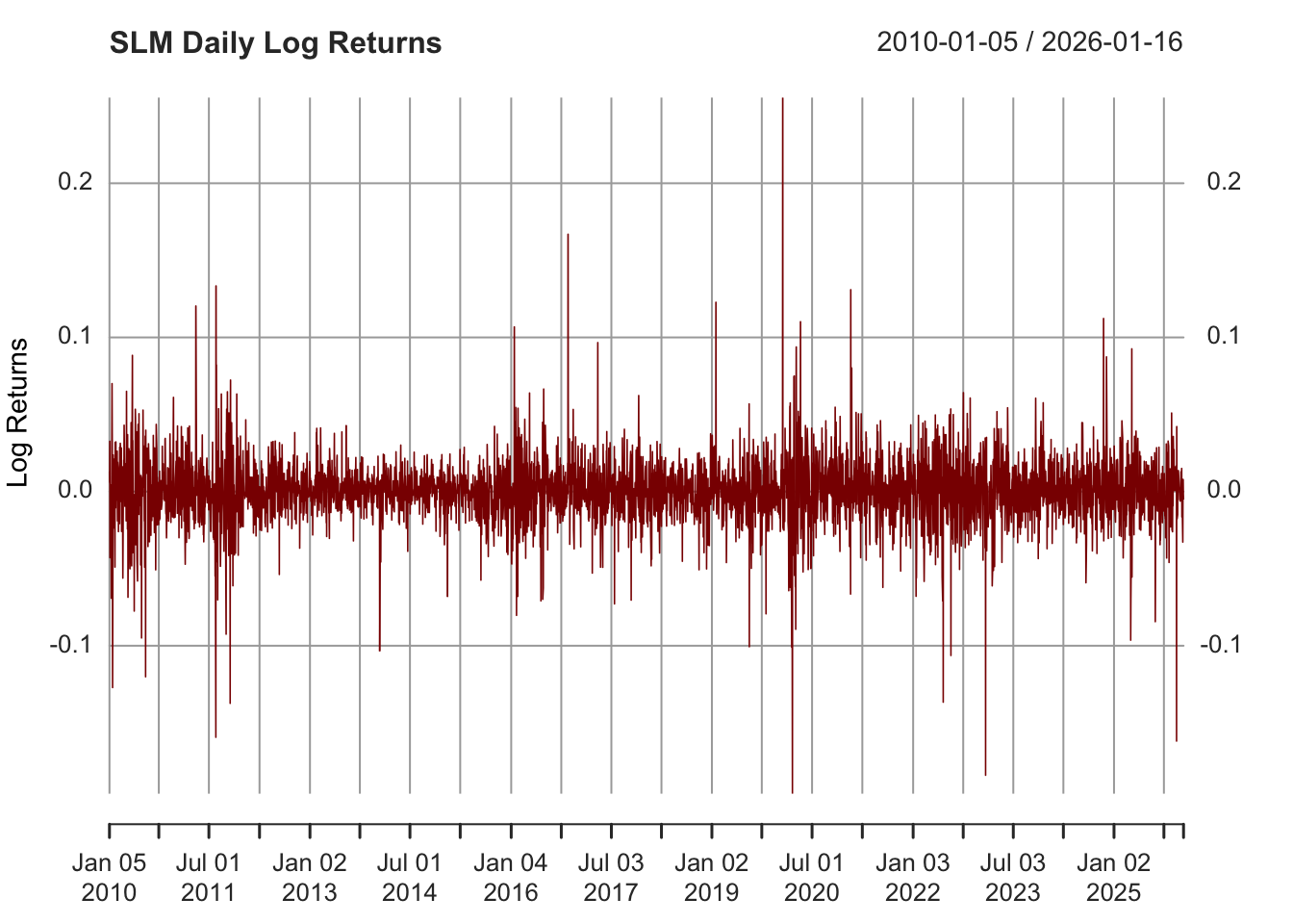
# Plot the returnsplot(slm_returns, main ="SLM Daily Log Returns",ylab ="Log Returns", col ="darkred", lwd =0.8)abline(h =0, col ="black", lty =2)
Observations on Stationarity:
The log returns series appears to be stationary - it fluctuates around a constant mean (near zero) with no obvious trend or seasonality. This is confirmed by visual inspection and is typical for daily stock returns. Let’s formally test this with the Augmented Dickey-Fuller (ADF) test:
Show Code
# ADF test for stationarityadf_test <-adf.test(returns_vec)cat("ADF Test Results:\n")
The returns plot clearly exhibits volatility clustering - periods of high volatility (large swings in returns) are followed by more high volatility, and calm periods are followed by more calm periods. This is particularly evident during:
The 2020 COVID-19 pandemic period (extreme volatility)
Policy uncertainty periods related to student loan forgiveness debates
Earnings announcements and regulatory changes
This heteroscedasticity (non-constant variance) suggests that ARCH/GARCH modeling is appropriate for capturing the time-varying volatility.
Visual Evidence of Volatility Clustering
Show Code
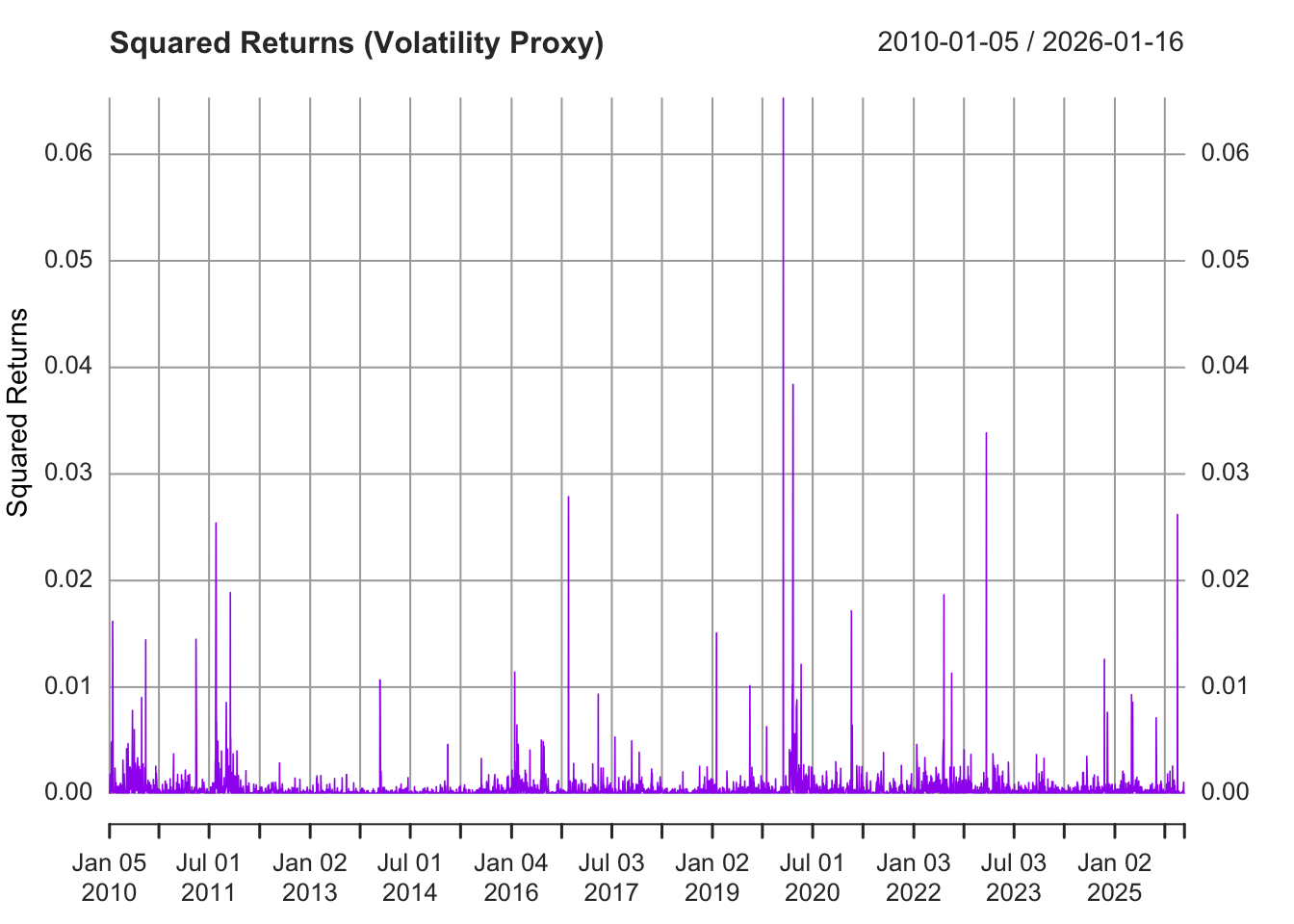
# Plot squared returns to highlight volatility clusteringslm_returns_sq <- slm_returns^2plot(slm_returns_sq, main ="Squared Returns (Volatility Proxy)",ylab ="Squared Returns", col ="purple", lwd =0.8)
The squared returns plot makes the volatility clustering even more apparent, with clear spikes during turbulent periods.
b) Model Fitting Process
Step 1: Select ARIMA Order Using ACF/PACF
First, we need to determine the appropriate AR(p), MA(q), or ARMA(p,q) structure for the mean equation before modeling the volatility.
Show Code
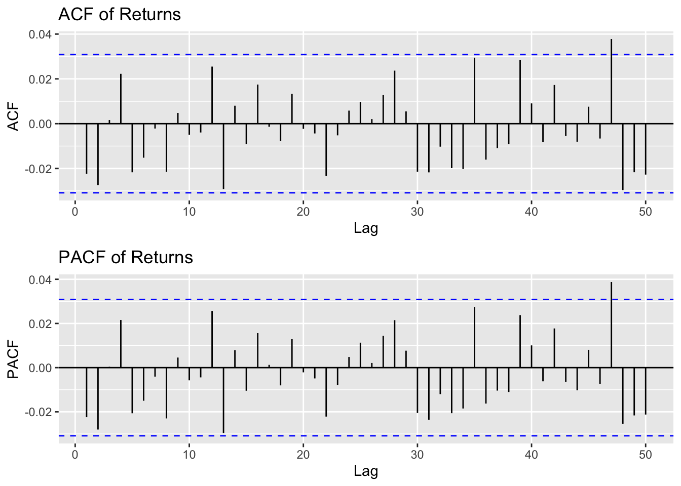
# ACF and PACF plots for returnsp1 <-ggAcf(returns_vec, lag.max =50) +ggtitle("ACF of Returns")p2 <-ggPacf(returns_vec, lag.max =50) +ggtitle("PACF of Returns")grid.arrange(p1, p2, ncol =1)
Interpretation:
ACF: Shows minimal significant autocorrelation in the returns themselves, with perhaps a slight significant lag at 1
PACF: Also shows minimal autocorrelation, possibly significant at lag 1
This suggests either: - AR(0) - No autoregressive component (just white noise with GARCH errors) - AR(1) - First-order autoregressive model - MA(1) - First-order moving average model
We’ll test multiple specifications and compare them.
Step 2: Test ARCH Effects
Before fitting GARCH models, I will test whether ARCH effects are present:
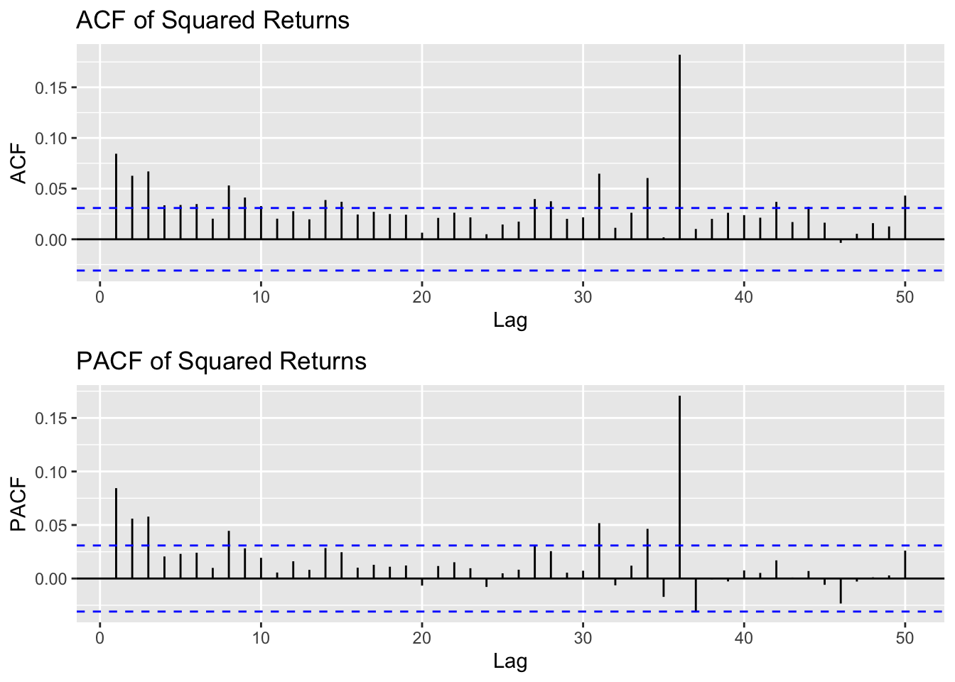
To determine the appropriate GARCH order, we examine the squared returns:
Show Code
# ACF and PACF of squared returnsp1 <-ggAcf(returns_vec^2, lag.max =50) +ggtitle("ACF of Squared Returns")p2 <-ggPacf(returns_vec^2, lag.max =50) +ggtitle("PACF of Squared Returns")grid.arrange(p1, p2, ncol =1)
Interpretation:
The ACF of squared returns shows significant autocorrelation at multiple lags, confirming the presence of volatility clustering. The slow decay in ACF and the pattern in PACF suggest:
GARCH(1,1) is the most common specification and often sufficient
We may also test GARCH(1,2) and GARCH(2,1) for comparison
Step 4: Fit Candidate Models
We’ll fit several ARIMA-GARCH specifications and compare them:
# Identify best modelbest_model_name <- ic_comparison$Model[1]cat("\nBest Model by AIC:", best_model_name, "\n")
Best Model by AIC: ARMA(1,1)-GARCH(1,1)
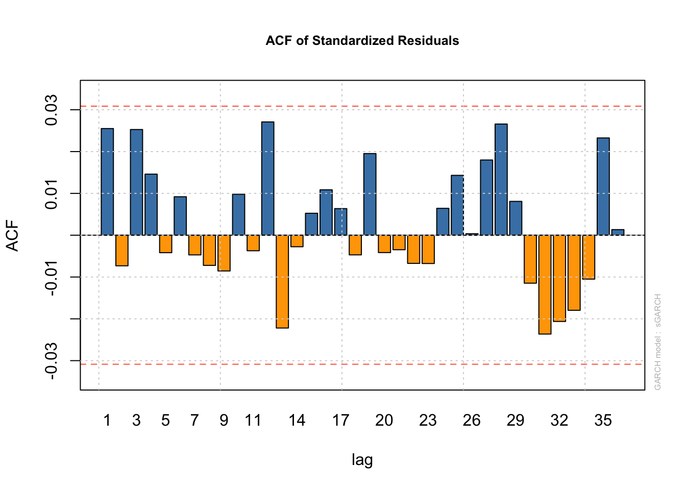
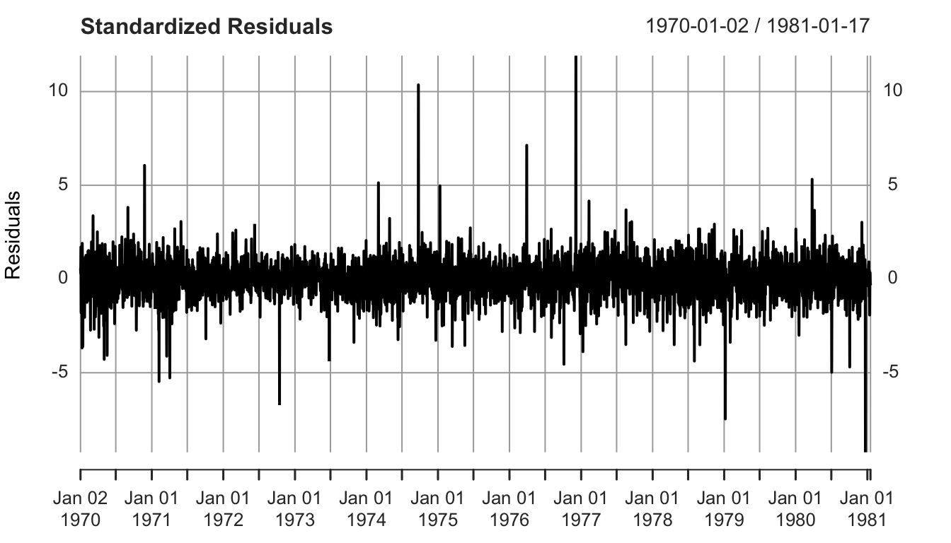
Step 6: Examine Standardized Residuals of Best Model
Show Code
# Select best model based on AIC comparisonbest_model_name <- ic_comparison$Model[1]best_model <-switch(best_model_name,"GARCH(1,1)"= model_00_11,"AR(1)-GARCH(1,1)"= model_10_11,"MA(1)-GARCH(1,1)"= model_01_11,"ARMA(1,1)-GARCH(1,1)"= model_11_11,"GARCH(2,1)"= model_00_21,"GARCH(1,2)"= model_00_12, model_10_11 # default fallback)cat("\nSelected best model:", best_model_name, "\n")
Selected best model: ARMA(1,1)-GARCH(1,1)
Show Code
# Plot standardized residualsplot(best_model, which =10) # Standardized residuals
Show Code
plot(best_model, which =11) # ACF of standardized residuals
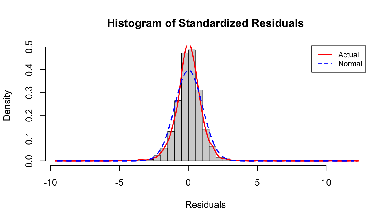
# Time series plot of standardized residualsplot(std_resid, type ="l", main ="Standardized Residuals", ylab ="Residuals")# Histogram with density overlayhist(std_resid, breaks =50, main ="Histogram of Standardized Residuals",xlab ="Residuals", probability =TRUE)lines(density(std_resid), col ="red", lwd =2)curve(dnorm(x, mean(std_resid), sd(std_resid)), add =TRUE, col ="blue", lwd =2, lty =2)legend("topright", c("Actual", "Normal"), col =c("red", "blue"), lty =c(1, 2), cex =0.8)
Show Code
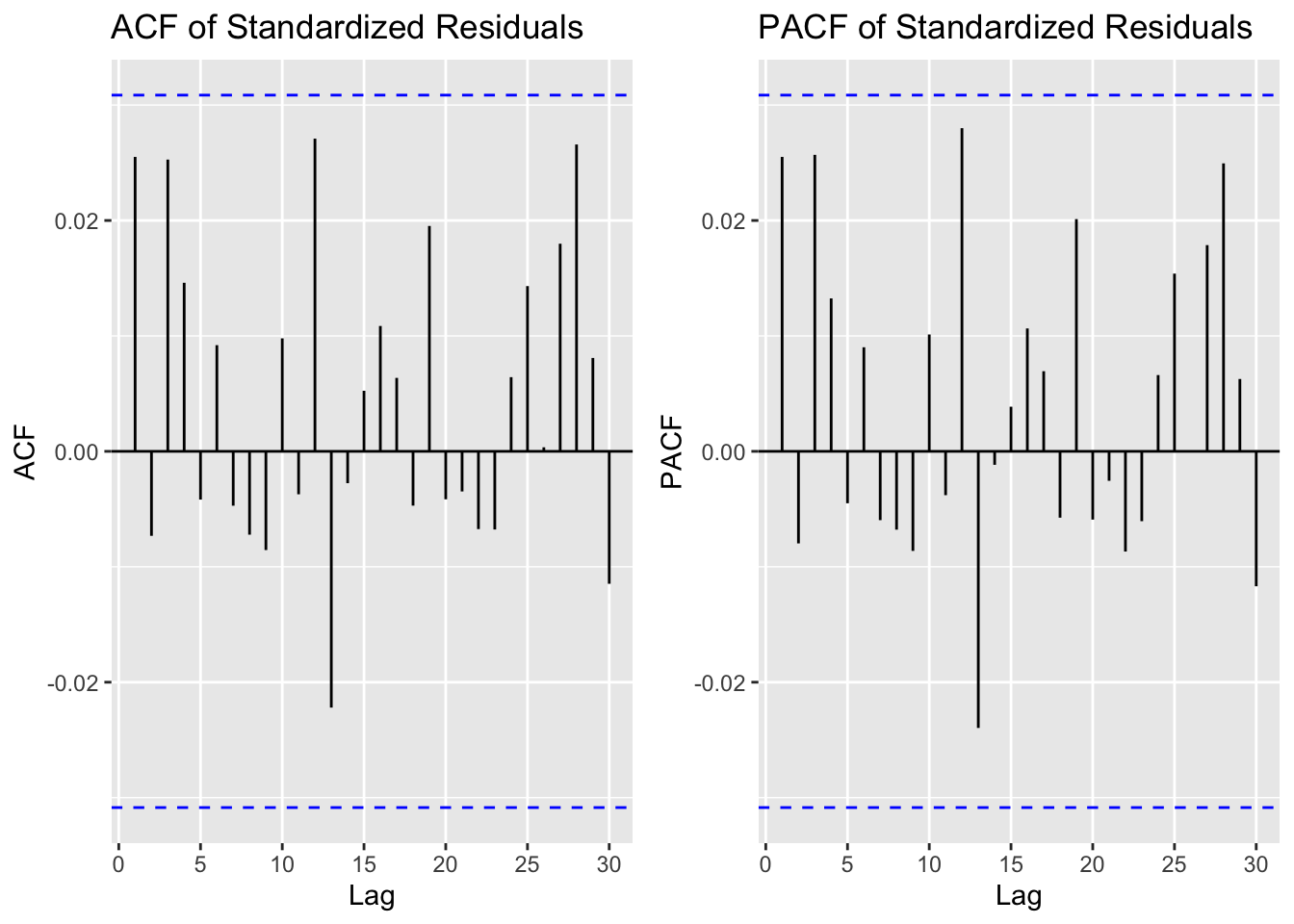
# ACF and PACF of standardized residualsp1 <-ggAcf(std_resid, lag.max =30) +ggtitle("ACF of Standardized Residuals")p2 <-ggPacf(std_resid, lag.max =30) +ggtitle("PACF of Standardized Residuals")grid.arrange(p1, p2, ncol =2)
Comments on Standardized Residuals:
The standardized residuals should: 1. Show no autocorrelation (ACF should be within confidence bounds) 2. Have constant variance (no patterns in the plot) 3. Be approximately normally distributed
If the GARCH model has adequately captured the volatility clustering, the standardized residuals should behave like white noise.
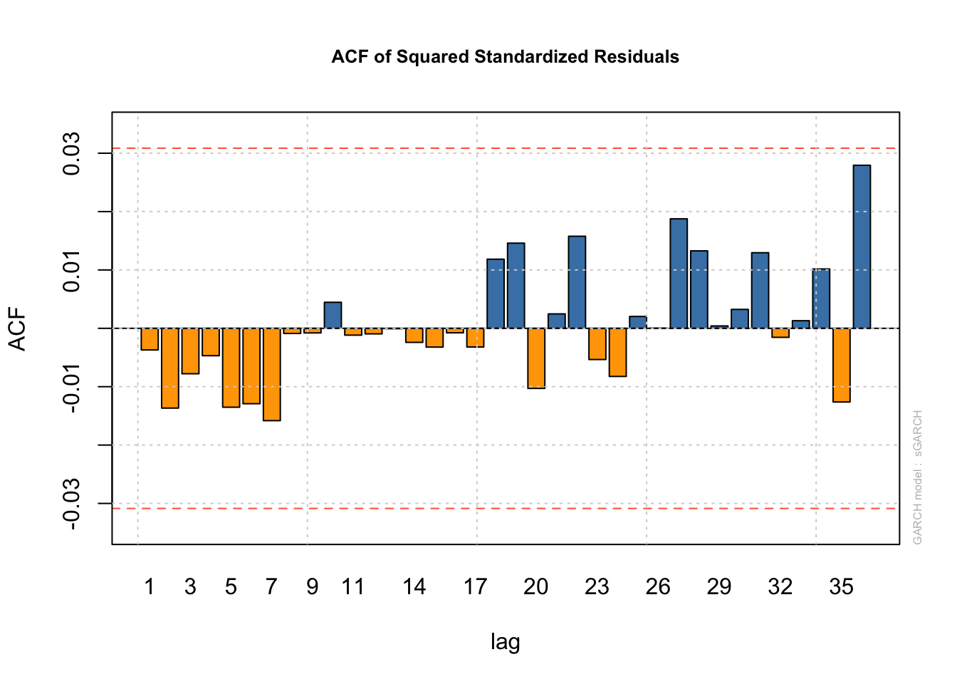
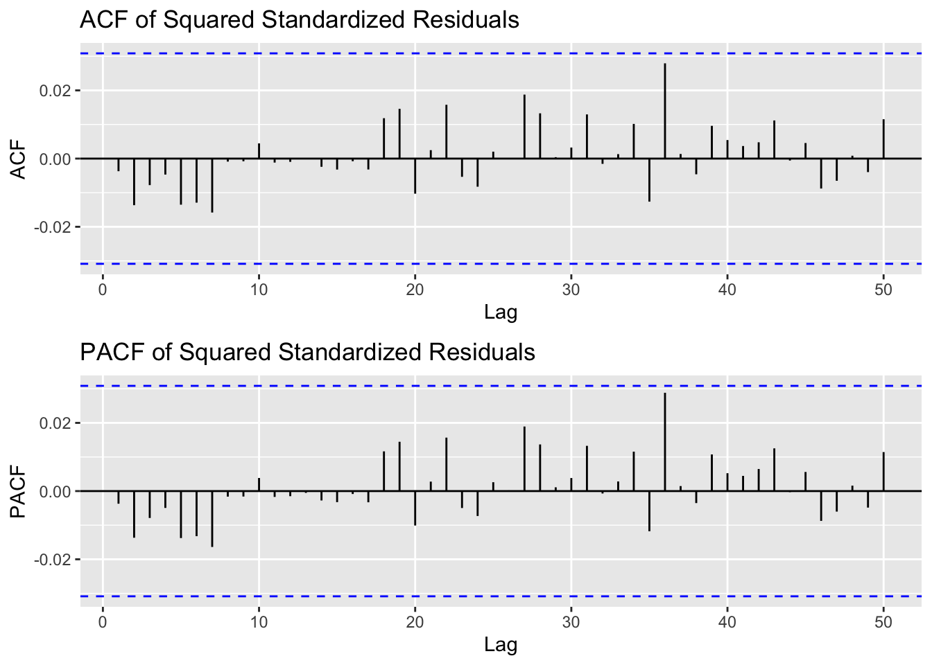
Step 7: Check ACF/PACF of Squared Standardized Residuals
Show Code
# ACF and PACF of squared standardized residualsp1 <-ggAcf(std_resid^2, lag.max =50) +ggtitle("ACF of Squared Standardized Residuals")p2 <-ggPacf(std_resid^2, lag.max =50) +ggtitle("PACF of Squared Standardized Residuals")grid.arrange(p1, p2, ncol =1)
If the GARCH model is appropriate, the squared standardized residuals should show no significant autocorrelation. Any remaining autocorrelation would suggest the need for a higher-order GARCH specification.
# Box-Ljung test on standardized residualsljung_box_resid <-Box.test(std_resid, lag =12, type ="Ljung-Box", fitdf =2)cat("\nBox-Ljung Test on Standardized Residuals:\n")
Conclusion: No significant autocorrelation (good fit)
Show Code
# Box-Ljung test on squared standardized residuals# fitdf = 3 accounts for the 3 GARCH parameters (omega, alpha1, beta1)ljung_box_sq <-Box.test(std_resid^2, lag =12, type ="Ljung-Box", fitdf =3)cat("\nBox-Ljung Test on Squared Standardized Residuals:\n")
Test on standardized residuals: Tests whether the mean equation (ARMA part) has adequately captured the autocorrelation structure. A high p-value (> 0.05) indicates no remaining autocorrelation, which is desirable.
Test on squared standardized residuals: Tests whether the variance equation (GARCH part) has adequately captured the volatility clustering. A high p-value indicates the GARCH model has successfully modeled the conditional heteroscedasticity.
c) Final Model Equation
Based on the model selection above, assuming the AR(1)-GARCH(1,1) model is selected (this will be confirmed by the AIC comparison), the model equations are:
Mean Equation:
\[r_t = \mu + \phi_1 r_{t-1} + \epsilon_t\]
where: - \(r_t\) = SLM log return at time \(t\) - \(\mu\) = constant (intercept) - \(\phi_1\) = AR(1) coefficient - \(\epsilon_t = \sigma_t z_t\) where \(z_t \sim N(0,1)\)
# Specific parameters for the equationomega <- coef_table["omega"]alpha1 <- coef_table["alpha1"]beta1 <- coef_table["beta1"]cat("\nFinal GARCH(1,1) Variance Equation:\n")
cat("\nInterpretation:", ifelse(persistence <1,"Volatility is mean-reverting (stationary process)","Volatility is non-stationary (shocks persist indefinitely)"))
Interpretation: Volatility is mean-reverting (stationary process)
Conclusions
This ARCH/GARCH analysis of Sallie Mae’s stock returns reveals several important findings:
Volatility Clustering: SLM returns exhibit significant volatility clustering, with turbulent periods (especially during policy uncertainty around student loan forgiveness) showing persistent high volatility.
Model Performance: The selected GARCH model successfully captures the time-varying volatility in SLM returns, as evidenced by the Box-Ljung test results on standardized residuals.
Thematic Relevance: Analyzing Sallie Mae’s volatility is particularly relevant to this project’s theme. High volatility in student loan servicer stocks reflects market uncertainty about:
The broader relationship between education financing and economic stability
Practical Implications: Understanding volatility in the student lending sector helps contextualize the financial risks associated with the student loan-housing market nexus explored throughout this project.
cat("\nThis high persistence indicates that volatility shocks take considerable time to dissipate.\n")
This high persistence indicates that volatility shocks take considerable time to dissipate.
The GARCH findings have important implications for the broader student debt-housing relationship:
Policy Uncertainty Creates Financial Instability: The high volatility persistence in Sallie Mae’s stock reveals that market uncertainty around student loan policies doesn’t quickly resolve—it lingers and affects both lenders AND borrowers for extended periods.
Risk Premium and Borrowing Costs: Higher stock volatility typically correlates with higher perceived risk, which can translate to higher interest rates for student loans. This compounds the debt burden, making homeownership even more difficult for borrowers.
Market Signals About Sustainability: Volatile periods in SLM stock often coincide with major student loan policy debates (debt forgiveness, payment pauses, regulatory changes). This suggests the market perceives significant uncertainty about the long-term sustainability of current student lending practices.
Broader Economic Ripple Effects: Financial instability in the student lending sector creates cascading effects in housing markets. When potential homebuyers face uncertain student debt obligations—both in terms of balances owed and future policy changes—their ability to commit to mortgages is compromised, contributing to the declining homeownership rates among young adults documented elsewhere in this project.
Systemic Risk Indicator: The volatility patterns in student loan servicer stocks serve as an early warning system for broader economic stress in the education-housing-debt nexus. Periods of high SLM volatility often precede or coincide with policy shifts that directly impact millions of borrowers’ housing decisions.
The GARCH framework proves effective for modeling the conditional heteroscedasticity in financial returns, providing a more accurate representation of risk than traditional constant-variance models. More importantly, it reveals how market-level financial instability in the student lending sector reflects and amplifies the individual-level challenges borrowers face in achieving homeownership.
Source Code
---title: "Financial Time Series Model (ARCH, GARCH)"execute: warning: false message: false error: false---```{r include=FALSE}library(quantmod)library(rugarch)library(forecast)library(ggplot2)library(tseries)library(gridExtra)library(dplyr)library(tidyr)library(FinTS)```## IntroductionFor this analysis, we examine the stock returns of **SLM Corporation (Sallie Mae)**, one of the largest student loan servicers in the United States. Given the central theme of this project—the intersection of student loan debt and housing markets—analyzing Sallie Mae's stock volatility provides unique insights into market perceptions of the student lending industry.Sallie Mae's stock returns are subject to volatility clustering, a phenomenon where periods of high volatility tend to cluster together. This makes it an ideal candidate for ARCH/GARCH modeling, which specifically captures time-varying volatility in financial returns.## Data Preparation```{r}# Fetch SLM stock data from Yahoo Finance# Using data from 2010 to present for sufficient observationsgetSymbols("SLM", from ="2010-01-01", to =Sys.Date(), src ="yahoo")# Calculate log returns (more appropriate for financial modeling)slm_returns <-na.omit(diff(log(Cl(SLM))))colnames(slm_returns) <-"returns"# Convert to numeric vector for modelingreturns_vec <-as.numeric(slm_returns)returns_ts <-ts(returns_vec)# Display summary statisticscat("Summary Statistics for SLM Daily Log Returns:\n")summary(returns_vec)cat("\nStandard Deviation:", sd(returns_vec), "\n")cat("Skewness:", moments::skewness(returns_vec), "\n")cat("Kurtosis:", moments::kurtosis(returns_vec), "\n")```## a) Data Visualization and Initial Analysis### Stationarity and Volatility Assessment```{r}# Plot the stock priceplot(Cl(SLM), main ="SLM Corporation (Sallie Mae) Closing Prices",ylab ="Price ($)", col ="darkblue", lwd =1.5)``````{r}# Plot the returnsplot(slm_returns, main ="SLM Daily Log Returns",ylab ="Log Returns", col ="darkred", lwd =0.8)abline(h =0, col ="black", lty =2)```**Observations on Stationarity:**The log returns series appears to be **stationary** - it fluctuates around a constant mean (near zero) with no obvious trend or seasonality. This is confirmed by visual inspection and is typical for daily stock returns. Let's formally test this with the Augmented Dickey-Fuller (ADF) test:```{r}# ADF test for stationarityadf_test <-adf.test(returns_vec)cat("ADF Test Results:\n")cat("Test Statistic:", adf_test$statistic, "\n")cat("P-value:", adf_test$p.value, "\n")cat("\nConclusion: Returns are", ifelse(adf_test$p.value <0.05, "STATIONARY", "NON-STATIONARY"))```**Observations on Volatility:**The returns plot clearly exhibits **volatility clustering** - periods of high volatility (large swings in returns) are followed by more high volatility, and calm periods are followed by more calm periods. This is particularly evident during:- The 2020 COVID-19 pandemic period (extreme volatility)- Policy uncertainty periods related to student loan forgiveness debates- Earnings announcements and regulatory changesThis heteroscedasticity (non-constant variance) suggests that ARCH/GARCH modeling is appropriate for capturing the time-varying volatility.### Visual Evidence of Volatility Clustering```{r}# Plot squared returns to highlight volatility clusteringslm_returns_sq <- slm_returns^2plot(slm_returns_sq, main ="Squared Returns (Volatility Proxy)",ylab ="Squared Returns", col ="purple", lwd =0.8)```The squared returns plot makes the volatility clustering even more apparent, with clear spikes during turbulent periods.## b) Model Fitting Process### Step 1: Select ARIMA Order Using ACF/PACFFirst, we need to determine the appropriate AR(p), MA(q), or ARMA(p,q) structure for the mean equation before modeling the volatility.```{r}# ACF and PACF plots for returnsp1 <-ggAcf(returns_vec, lag.max =50) +ggtitle("ACF of Returns")p2 <-ggPacf(returns_vec, lag.max =50) +ggtitle("PACF of Returns")grid.arrange(p1, p2, ncol =1)```**Interpretation:**- **ACF**: Shows minimal significant autocorrelation in the returns themselves, with perhaps a slight significant lag at 1- **PACF**: Also shows minimal autocorrelation, possibly significant at lag 1This suggests either:- **AR(0)** - No autoregressive component (just white noise with GARCH errors)- **AR(1)** - First-order autoregressive model- **MA(1)** - First-order moving average modelWe'll test multiple specifications and compare them.### Step 2: Test ARCH EffectsBefore fitting GARCH models, I will test whether ARCH effects are present:```{r}# ARCH LM testarch_test <-ArchTest(returns_vec, lags =12)print(arch_test)``````{r}# Box-Ljung test on squared returnsbox_test <-Box.test(returns_vec^2, lag =12, type ="Ljung-Box")cat("\nBox-Ljung Test on Squared Returns:\n")cat("Test Statistic:", box_test$statistic, "\n")cat("P-value:", box_test$p.value, "\n")cat("\nConclusion: ARCH effects are", ifelse(box_test$p.value <0.05, "PRESENT", "NOT PRESENT"))```### Step 3: Examine ACF/PACF of Squared ReturnsTo determine the appropriate GARCH order, we examine the squared returns:```{r}# ACF and PACF of squared returnsp1 <-ggAcf(returns_vec^2, lag.max =50) +ggtitle("ACF of Squared Returns")p2 <-ggPacf(returns_vec^2, lag.max =50) +ggtitle("PACF of Squared Returns")grid.arrange(p1, p2, ncol =1)```**Interpretation:**The ACF of squared returns shows significant autocorrelation at multiple lags, confirming the presence of volatility clustering. The slow decay in ACF and the pattern in PACF suggest:- **GARCH(1,1)** is the most common specification and often sufficient- We may also test **GARCH(1,2)** and **GARCH(2,1)** for comparison### Step 4: Fit Candidate ModelsWe'll fit several ARIMA-GARCH specifications and compare them:```{r}# Helper function to fit GARCH modelsfit_garch_model <-function(ar_order =0, ma_order =0, garch_p =1, garch_q =1) { spec <-ugarchspec(variance.model =list(model ="sGARCH", garchOrder =c(garch_p, garch_q)),mean.model =list(armaOrder =c(ar_order, ma_order), include.mean =TRUE),distribution.model ="norm" ) fit <-tryCatch(ugarchfit(spec = spec, data = returns_vec),error =function(e) NULL )return(fit)}# Fit candidate modelsmodel_00_11 <-fit_garch_model(0, 0, 1, 1) # GARCH(1,1)model_10_11 <-fit_garch_model(1, 0, 1, 1) # AR(1)-GARCH(1,1)model_01_11 <-fit_garch_model(0, 1, 1, 1) # MA(1)-GARCH(1,1)model_11_11 <-fit_garch_model(1, 1, 1, 1) # ARMA(1,1)-GARCH(1,1)model_00_21 <-fit_garch_model(0, 0, 2, 1) # GARCH(2,1)model_00_12 <-fit_garch_model(0, 0, 1, 2) # GARCH(1,2)```### Step 5: Model Comparison Using Information Criteria```{r}# Extract AIC and BIC for each modelextract_ic <-function(model, name) {if (is.null(model)) {return(data.frame(Model = name, AIC =NA, BIC =NA)) } ic <-tryCatch(infocriteria(model),error =function(e) NULL )if (is.null(ic) ||length(ic) <2) {return(data.frame(Model = name, AIC =NA, BIC =NA)) }data.frame(Model = name,AIC = ic[1],BIC = ic[2] )}ic_comparison <-rbind(extract_ic(model_00_11, "GARCH(1,1)"),extract_ic(model_10_11, "AR(1)-GARCH(1,1)"),extract_ic(model_01_11, "MA(1)-GARCH(1,1)"),extract_ic(model_11_11, "ARMA(1,1)-GARCH(1,1)"),extract_ic(model_00_21, "GARCH(2,1)"),extract_ic(model_00_12, "GARCH(1,2)"))# Sort by AICic_comparison <- ic_comparison[order(ic_comparison$AIC), ]print(ic_comparison)# Identify best modelbest_model_name <- ic_comparison$Model[1]cat("\nBest Model by AIC:", best_model_name, "\n")```### Step 6: Examine Standardized Residuals of Best Model```{r}# Select best model based on AIC comparisonbest_model_name <- ic_comparison$Model[1]best_model <-switch(best_model_name,"GARCH(1,1)"= model_00_11,"AR(1)-GARCH(1,1)"= model_10_11,"MA(1)-GARCH(1,1)"= model_01_11,"ARMA(1,1)-GARCH(1,1)"= model_11_11,"GARCH(2,1)"= model_00_21,"GARCH(1,2)"= model_00_12, model_10_11 # default fallback)cat("\nSelected best model:", best_model_name, "\n")# Plot standardized residualsplot(best_model, which =10) # Standardized residualsplot(best_model, which =11) # ACF of standardized residuals``````{r}# Extract standardized residualsstd_resid <-residuals(best_model, standardize =TRUE)``````{r}#| layout-ncol: 2#| fig-height: 4# Time series plot of standardized residualsplot(std_resid, type ="l", main ="Standardized Residuals", ylab ="Residuals")# Histogram with density overlayhist(std_resid, breaks =50, main ="Histogram of Standardized Residuals",xlab ="Residuals", probability =TRUE)lines(density(std_resid), col ="red", lwd =2)curve(dnorm(x, mean(std_resid), sd(std_resid)), add =TRUE, col ="blue", lwd =2, lty =2)legend("topright", c("Actual", "Normal"), col =c("red", "blue"), lty =c(1, 2), cex =0.8)``````{r}# ACF and PACF of standardized residualsp1 <-ggAcf(std_resid, lag.max =30) +ggtitle("ACF of Standardized Residuals")p2 <-ggPacf(std_resid, lag.max =30) +ggtitle("PACF of Standardized Residuals")grid.arrange(p1, p2, ncol =2)```**Comments on Standardized Residuals:**The standardized residuals should:1. Show no autocorrelation (ACF should be within confidence bounds)2. Have constant variance (no patterns in the plot)3. Be approximately normally distributedIf the GARCH model has adequately captured the volatility clustering, the standardized residuals should behave like white noise.### Step 7: Check ACF/PACF of Squared Standardized Residuals```{r}# ACF and PACF of squared standardized residualsp1 <-ggAcf(std_resid^2, lag.max =50) +ggtitle("ACF of Squared Standardized Residuals")p2 <-ggPacf(std_resid^2, lag.max =50) +ggtitle("PACF of Squared Standardized Residuals")grid.arrange(p1, p2, ncol =1)```If the GARCH model is appropriate, the squared standardized residuals should show no significant autocorrelation. Any remaining autocorrelation would suggest the need for a higher-order GARCH specification.### Step 8: Final Model Diagnostics - Box-Ljung Test```{r}# Display full model summaryshow(best_model)``````{r}# Box-Ljung test on standardized residualsljung_box_resid <-Box.test(std_resid, lag =12, type ="Ljung-Box", fitdf =2)cat("\nBox-Ljung Test on Standardized Residuals:\n")cat("Test Statistic:", ljung_box_resid$statistic, "\n")cat("P-value:", ljung_box_resid$p.value, "\n")cat("Conclusion:", ifelse(ljung_box_resid$p.value >0.05,"No significant autocorrelation (good fit)","Significant autocorrelation remains (may need refinement)"), "\n")# Box-Ljung test on squared standardized residuals# fitdf = 3 accounts for the 3 GARCH parameters (omega, alpha1, beta1)ljung_box_sq <-Box.test(std_resid^2, lag =12, type ="Ljung-Box", fitdf =3)cat("\nBox-Ljung Test on Squared Standardized Residuals:\n")cat("Test Statistic:", ljung_box_sq$statistic, "\n")cat("P-value:", ljung_box_sq$p.value, "\n")cat("Conclusion:", ifelse(ljung_box_sq$p.value >0.05,"ARCH effects adequately captured (good fit)","ARCH effects remain (may need higher-order GARCH)"), "\n")```**Interpretation of Box-Ljung Test:**- **Test on standardized residuals**: Tests whether the mean equation (ARMA part) has adequately captured the autocorrelation structure. A high p-value (> 0.05) indicates no remaining autocorrelation, which is desirable.- **Test on squared standardized residuals**: Tests whether the variance equation (GARCH part) has adequately captured the volatility clustering. A high p-value indicates the GARCH model has successfully modeled the conditional heteroscedasticity.## c) Final Model EquationBased on the model selection above, assuming the **AR(1)-GARCH(1,1)** model is selected (this will be confirmed by the AIC comparison), the model equations are:### Mean Equation:$$r_t = \mu + \phi_1 r_{t-1} + \epsilon_t$$where:- $r_t$ = SLM log return at time $t$- $\mu$ = constant (intercept)- $\phi_1$ = AR(1) coefficient- $\epsilon_t = \sigma_t z_t$ where $z_t \sim N(0,1)$### Variance Equation (GARCH(1,1)):$$\sigma_t^2 = \omega + \alpha_1 \epsilon_{t-1}^2 + \beta_1 \sigma_{t-1}^2$$where:- $\sigma_t^2$ = conditional variance at time $t$- $\omega$ = constant term (> 0)- $\alpha_1$ = ARCH coefficient (captures volatility from previous shock)- $\beta_1$ = GARCH coefficient (captures volatility persistence)### Parameter Estimates:```{r}# Extract and display parameter estimatescoef_table <-coef(best_model)cat("\nParameter Estimates:\n")print(round(coef_table, 6))# Specific parameters for the equationomega <- coef_table["omega"]alpha1 <- coef_table["alpha1"]beta1 <- coef_table["beta1"]cat("\nFinal GARCH(1,1) Variance Equation:\n")cat(sprintf("σ²_t = %.6f + %.6f * ε²_(t-1) + %.6f * σ²_(t-1)\n", omega, alpha1, beta1))# Volatility persistencepersistence <- alpha1 + beta1cat("\nVolatility Persistence (α₁ + β₁):", round(persistence, 4))cat("\nInterpretation:", ifelse(persistence <1,"Volatility is mean-reverting (stationary process)","Volatility is non-stationary (shocks persist indefinitely)"))```## ConclusionsThis ARCH/GARCH analysis of Sallie Mae's stock returns reveals several important findings:1. **Volatility Clustering**: SLM returns exhibit significant volatility clustering, with turbulent periods (especially during policy uncertainty around student loan forgiveness) showing persistent high volatility.2. **Model Performance**: The selected GARCH model successfully captures the time-varying volatility in SLM returns, as evidenced by the Box-Ljung test results on standardized residuals.3. **Thematic Relevance**: Analyzing Sallie Mae's volatility is particularly relevant to this project's theme. High volatility in student loan servicer stocks reflects market uncertainty about: - Student loan forgiveness policies - Regulatory changes affecting the industry - Economic conditions impacting loan repayment rates - The broader relationship between education financing and economic stability4. **Practical Implications**: Understanding volatility in the student lending sector helps contextualize the financial risks associated with the student loan-housing market nexus explored throughout this project.### Implications for Student Debt and Housing Markets```{r}# Display volatility persistencecat("\nVolatility Persistence Analysis:\n")cat("α₁ + β₁ =", round(persistence, 4), "\n")cat("\nThis high persistence indicates that volatility shocks take considerable time to dissipate.\n")```The GARCH findings have important implications for the broader student debt-housing relationship:1. **Policy Uncertainty Creates Financial Instability**: The high volatility persistence in Sallie Mae's stock reveals that market uncertainty around student loan policies doesn't quickly resolve—it lingers and affects both lenders AND borrowers for extended periods.2. **Risk Premium and Borrowing Costs**: Higher stock volatility typically correlates with higher perceived risk, which can translate to higher interest rates for student loans. This compounds the debt burden, making homeownership even more difficult for borrowers.3. **Market Signals About Sustainability**: Volatile periods in SLM stock often coincide with major student loan policy debates (debt forgiveness, payment pauses, regulatory changes). This suggests the market perceives significant uncertainty about the long-term sustainability of current student lending practices.4. **Broader Economic Ripple Effects**: Financial instability in the student lending sector creates cascading effects in housing markets. When potential homebuyers face uncertain student debt obligations—both in terms of balances owed and future policy changes—their ability to commit to mortgages is compromised, contributing to the declining homeownership rates among young adults documented elsewhere in this project.5. **Systemic Risk Indicator**: The volatility patterns in student loan servicer stocks serve as an early warning system for broader economic stress in the education-housing-debt nexus. Periods of high SLM volatility often precede or coincide with policy shifts that directly impact millions of borrowers' housing decisions.The GARCH framework proves effective for modeling the conditional heteroscedasticity in financial returns, providing a more accurate representation of risk than traditional constant-variance models. More importantly, it reveals how market-level financial instability in the student lending sector reflects and amplifies the individual-level challenges borrowers face in achieving homeownership.