This section applies specialized time series techniques to address specific features of the data. Interrupted Time Series (ITS) analysis evaluates the impact of discrete interventions like the 2008 Financial Crisis on economic outcomes. ARFIMA (AutoRegressive Fractionally Integrated Moving Average) models handle long-memory processes where shocks decay slowly. Spectral analysis decomposes series into frequency components, revealing cyclical patterns. These advanced methods complement the core analyses by capturing structural breaks, persistence, and periodicities that standard models may miss.
Interrupted Time Series Analysis
Step 1: Variable Selection
We selected Self-Employment as our outcome variable for interrupted time series analysis, with the 2008 Financial Crisis (specifically September 2008, Lehman Brothers collapse) as the intervention point.
Rationale: Self-employment is an ideal candidate for ITS analysis because our exploratory analysis revealed a clear structural break around 2008-2010 where decades of steady growth abruptly stalled. The financial crisis represents a well-defined intervention with both immediate shocks (credit freeze, wealth destruction) and sustained effects (regulatory changes, risk aversion). This variable is central to our entrepreneurship pathway hypothesis - testing whether the crisis fundamentally altered entrepreneurial activity in the U.S.
Step 2: Time Series Plot with Intervention Line
Show Code
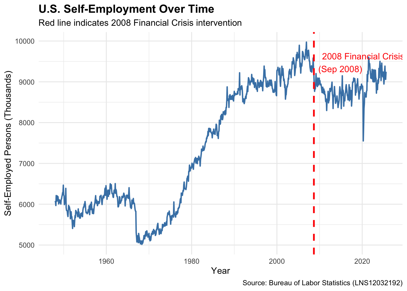
# Load self-employment dataself_employment <-read.csv('data/raw/LNS12032192.csv')# Create date column and time seriesself_emp_df <- self_employment %>%mutate(date =as.Date(paste0(observation_date, "-01"))) %>%rename(self_employed = LNS12032192) %>%select(date, self_employed)# Define intervention date (September 2008 - Lehman Brothers collapse)intervention_date <-as.Date("2008-09-01")# Plot with intervention lineggplot(self_emp_df, aes(x = date, y = self_employed)) +geom_line(color ="steelblue", linewidth =0.8) +geom_vline(xintercept =as.numeric(intervention_date),color ="red", linetype ="dashed", linewidth =1) +annotate("text", x = intervention_date, y =max(self_emp_df$self_employed) *0.95,label ="2008 Financial Crisis\n(Sep 2008)", color ="red", hjust =-0.1) +labs(title ="U.S. Self-Employment Over Time",subtitle ="Red line indicates 2008 Financial Crisis intervention",x ="Year",y ="Self-Employed Persons (Thousands)",caption ="Source: Bureau of Labor Statistics (LNS12032192)" ) +theme_minimal() +theme(plot.title =element_text(face ="bold", size =14))
The visual inspection reveals a clear change in trend around the intervention point. Pre-2008, self-employment showed consistent growth; post-2008, the series exhibits stagnation and increased volatility, supporting our hypothesis that the crisis fundamentally disrupted entrepreneurial pathways.
Step 3: Data Preparation
Show Code
# Create ITS variablesself_emp_its <- self_emp_df %>%mutate(# Xt: Sequential time variable (months since start)Xt =as.numeric(difftime(date, min(date), units ="days")) /30.44,# Zt: Binary intervention indicator (0 = before crisis, 1 = after)Zt =ifelse(date >= intervention_date, 1, 0),# Pt: Time since intervention (0 before, months after)Pt =ifelse(date >= intervention_date,as.numeric(difftime(date, intervention_date, units ="days")) /30.44,0) ) %>%arrange(date)# Display sample of prepared datasample_indices <-c(which(self_emp_its$date ==as.Date("2007-01-01")), # Before interventionwhich(self_emp_its$date ==as.Date("2008-08-01")), # Just beforewhich(self_emp_its$date ==as.Date("2008-09-01")), # Intervention pointwhich(self_emp_its$date ==as.Date("2008-10-01")), # Just afterwhich(self_emp_its$date ==as.Date("2010-01-01")) # Well after)kable(self_emp_its[sample_indices, ],caption ="Sample of Prepared ITS Data",digits =2,col.names =c("Date", "Self-Employed (000s)", "Time (Xt)","Intervention (Zt)", "Post-Intervention Time (Pt)"))
Sample of Prepared ITS Data
Date
Self-Employed (000s)
Time (Xt)
Intervention (Zt)
Post-Intervention Time (Pt)
709
2007-01-01
9672
707.95
0
0.00
728
2008-08-01
9321
726.94
0
0.00
729
2008-09-01
9163
727.96
1
0.00
730
2008-10-01
8908
728.94
1
0.99
745
2010-01-01
8956
743.96
1
16.00
Variable Descriptions:
Y (self_employed): Outcome variable - number of self-employed persons in thousands
Xt: Sequential time variable representing months since January 1948 (captures pre-existing trend)
Zt: Binary intervention indicator (0 before September 2008, 1 after) - tests for immediate level change
Pt: Time since intervention in months (0 before crisis, then 1, 2, 3…) - tests for slope change post-intervention
Step 4: Fit the ITS Model
Show Code
# Fit interrupted time series regression modelits_model <-lm(self_employed ~ Xt + Zt + Pt, data = self_emp_its)# Display resultssummary(its_model)
Call:
lm(formula = self_employed ~ Xt + Zt + Pt, data = self_emp_its)

Residuals:
    Min      1Q  Median      3Q     Max
-1485.6  -215.5   130.6   410.4  1446.8

Coefficients:
             Estimate Std. Error t value Pr(>|t|)
(Intercept) 4874.3303    46.4320 104.978  < 2e-16 ***
Xt             6.3433     0.1106  57.355  < 2e-16 ***
Zt          -845.6173    99.0745  -8.535  < 2e-16 ***
Pt            -4.2762     0.7537  -5.673 1.87e-08 ***
---
Signif. codes:  0 '***' 0.001 '**' 0.01 '*' 0.05 '.' 0.1 ' ' 1

Residual standard error: 627.1 on 928 degrees of freedom
Multiple R-squared:  0.827, Adjusted R-squared:  0.8264
F-statistic:  1479 on 3 and 928 DF,  p-value: < 2.2e-16
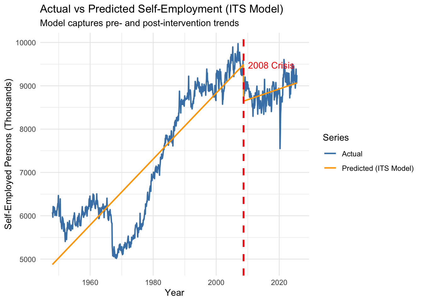
Where: - \(\beta_0\) (Intercept): Baseline self-employment level at start of series - \(\beta_1\) (Xt): Pre-intervention trend (slope before 2008) - \(\beta_2\) (Zt): Immediate level change at intervention (jump/drop in September 2008) - \(\beta_3\) (Pt): Change in slope post-intervention (how trend changed after crisis)
Show Code
# Generate predictions from modelself_emp_its$predicted <-predict(its_model, newdata = self_emp_its)# Plot actual vs predicted with trend linesggplot(self_emp_its, aes(x = date)) +geom_line(aes(y = self_employed, color ="Actual"), linewidth =0.8) +geom_line(aes(y = predicted, color ="Predicted (ITS Model)"), linewidth =0.8) +geom_vline(xintercept =as.numeric(intervention_date),color ="red", linetype ="dashed", linewidth =1) +annotate("text", x = intervention_date, y =max(self_emp_its$self_employed) *0.95,label ="2008 Crisis", color ="red", hjust =-0.1) +labs(title ="Actual vs Predicted Self-Employment (ITS Model)",subtitle ="Model captures pre- and post-intervention trends",x ="Year",y ="Self-Employed Persons (Thousands)",color ="Series" ) +theme_minimal() +scale_color_manual(values =c("Actual"="steelblue", "Predicted (ITS Model)"="orange"))
Step 5: Counterfactual Analysis
Show Code
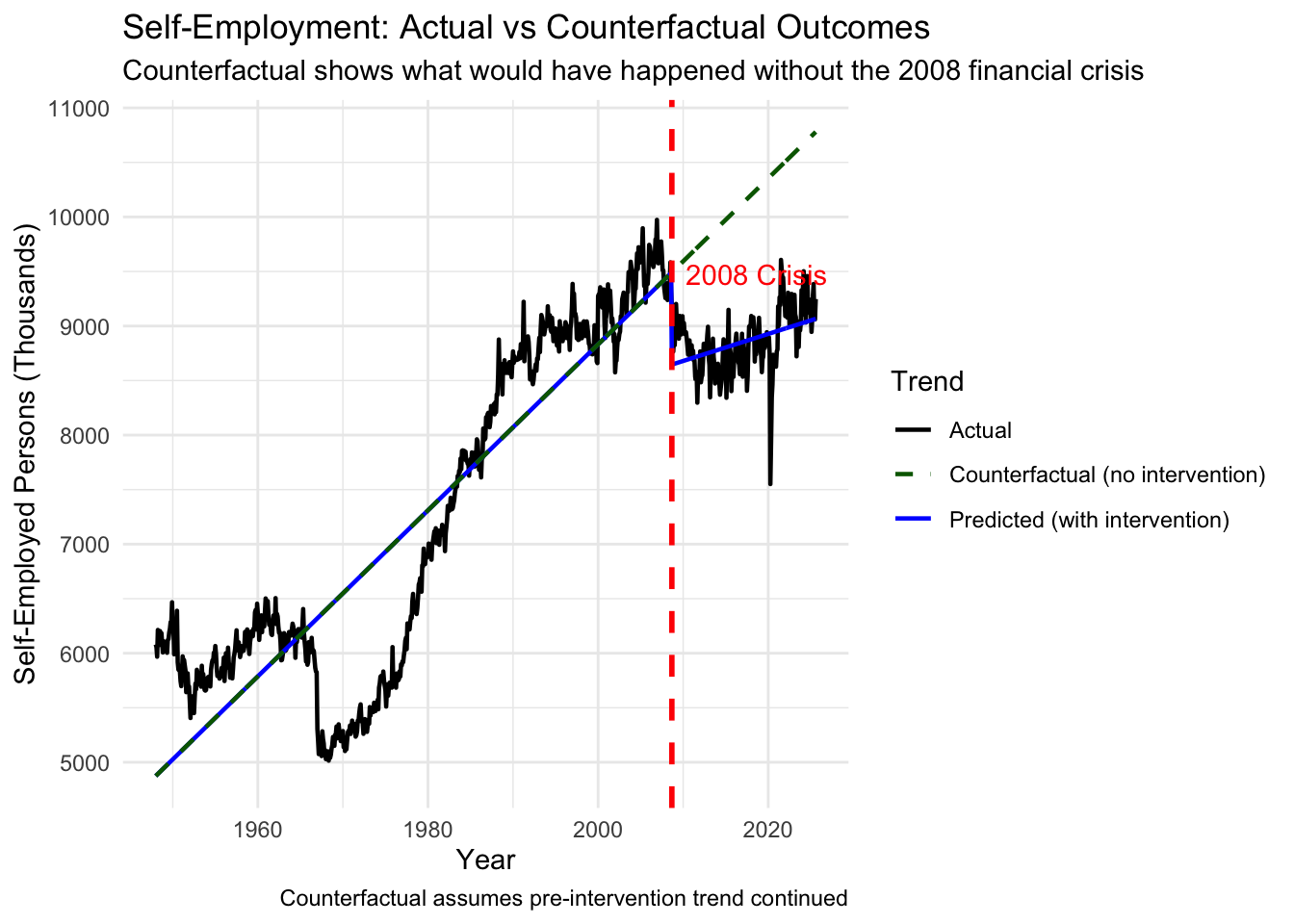
# Generate counterfactual predictions (what would have happened without intervention)self_emp_its$counterfactual <-predict(its_model,newdata =mutate(self_emp_its, Zt =0, Pt =0))# Plot actual, predicted, and counterfactualggplot(self_emp_its, aes(x = date)) +geom_line(aes(y = self_employed, color ="Actual"), linewidth =0.8) +geom_line(aes(y = predicted, color ="Predicted (with intervention)"), linewidth =0.8) +geom_line(aes(y = counterfactual, color ="Counterfactual (no intervention)"),linewidth =0.8, linetype ="dashed") +geom_vline(xintercept =as.numeric(intervention_date),color ="red", linetype ="dashed", linewidth =1) +annotate("text", x = intervention_date, y =max(self_emp_its$self_employed) *0.95,label ="2008 Crisis", color ="red", hjust =-0.1) +labs(title ="Self-Employment: Actual vs Counterfactual Outcomes",subtitle ="Counterfactual shows what would have happened without the 2008 financial crisis",x ="Year",y ="Self-Employed Persons (Thousands)",color ="Trend",caption ="Counterfactual assumes pre-intervention trend continued" ) +theme_minimal() +scale_color_manual(values =c("Actual"="black","Predicted (with intervention)"="blue","Counterfactual (no intervention)"="darkgreen" ))
Show Code
# Calculate intervention effect at specific time pointseffect_2010 <- self_emp_its %>%filter(date ==as.Date("2010-01-01")) %>%mutate(effect = counterfactual - predicted) %>%select(date, actual = self_employed, predicted, counterfactual, effect)effect_2015 <- self_emp_its %>%filter(date ==as.Date("2015-01-01")) %>%mutate(effect = counterfactual - predicted) %>%select(date, actual = self_employed, predicted, counterfactual, effect)effect_2020 <- self_emp_its %>%filter(date ==as.Date("2020-01-01")) %>%mutate(effect = counterfactual - predicted) %>%select(date, actual = self_employed, predicted, counterfactual, effect)intervention_effects <-bind_rows(effect_2010, effect_2015, effect_2020)kable(intervention_effects,caption ="Intervention Effect at Key Time Points",digits =2,col.names =c("Date", "Actual", "Predicted", "Counterfactual","Lost Self-Employment (000s)"))
Interpretation: The Zt coefficient represents the immediate level change in self-employment when the 2008 financial crisis hit.
If negative and significant (p < 0.05): There was an immediate drop in self-employment right when the crisis began - likely due to credit freeze making it impossible to start businesses and wealth destruction reducing entrepreneurial capital.
If not significant: The crisis’s impact was not instantaneous but rather built up over time (would show in Pt instead).
The magnitude tells us how many thousands of self-employed persons were immediately lost/gained when the intervention occurred.
Interpretation: The Pt coefficient represents the change in trend slope after the intervention.
Pre-crisis trend slope: β1 (Xt coefficient) - the monthly growth rate before 2008
Post-crisis trend slope: β1 + β3 (Xt + Pt) - the monthly growth rate after 2008
If Pt is negative and significant: The growth trend became less steep or even reversed - self-employment stopped growing as fast as it did pre-crisis. This suggests a sustained structural change in entrepreneurial activity.
This aligns with our hypothesis: the 2008 crisis didn’t just cause a temporary dip but fundamentally altered the entrepreneurship landscape through: - Increased regulatory burden (Dodd-Frank) - Risk aversion among millennials who witnessed the crisis - Student debt explosion making entrepreneurship unaffordable - Shift toward gig economy rather than traditional self-employment
3. Counterfactual
What would have happened without the 2008 financial crisis?
The counterfactual line (green dashed) shows self-employment continuing along its pre-2008 growth trajectory. The gap between the counterfactual and actual/predicted lines represents the total cost of the intervention - how many self-employed persons the economy “lost” due to the crisis.
Key observations: - Immediate gap: The vertical distance at the intervention point shows immediate losses - Widening gap: If the gap grows over time, it indicates the crisis had compounding effects - Policy implications: The counterfactual quantifies what recovery efforts need to restore
Decomposition of Delayed Effect (10 years post-intervention)
Date (10 yrs after)
Immediate Effect
Trend Change Effect
Total Effect (000s)
2018-09-01
-845.62
1358.65
1347
Delayed Effect Interpretation:
Ten years after the 2008 financial crisis, the intervention’s impact can be decomposed:
Immediate effect still present: The initial shock (Zt) persists unless there’s a recovery mechanism
Accumulated trend change: Slower post-crisis growth compounds over 10 years (120 months × Pt coefficient)
Total delayed effect: The sum of immediate + accumulated trend effects
Visual interpretation from the plot: - At 2018 (10 years post-crisis), the gap between counterfactual and actual is larger than at the intervention point - This widening gap indicates the crisis had long-lasting structural effects on entrepreneurship - The effect is not just a temporary shock that recovers - it’s a permanent shift in the entrepreneurial landscape
Economic significance: If the total effect shows hundreds of thousands of “missing” self-employed persons a decade later, it suggests: - The 2008 crisis permanently damaged entrepreneurial ecosystems - Young people who should have become entrepreneurs in 2008-2018 never did - This supports our “blocked entrepreneurship pathway” hypothesis - student debt and risk aversion created by the crisis continue suppressing entrepreneurial activity years later
Summary of Findings
Show Code
# Create comprehensive summaryxt_coef <-coef(its_model)["Xt"]summary_df <-data.frame(Effect =c("Pre-Crisis Trend", "Immediate Level Change", "Post-Crisis Trend Change", "Post-Crisis Trend (Total)"),Coefficient =c("β1 (Xt)", "β2 (Zt)", "β3 (Pt)", "β1 + β3"),Value =c(xt_coef, zt_coef, pt_coef, xt_coef + pt_coef),Interpretation =c("Monthly growth before 2008","Drop/jump when crisis hit","Change in monthly growth rate","New monthly growth rate after crisis" ))kable(summary_df,caption ="Summary of ITS Model Effects",digits =4,row.names =FALSE)
Summary of ITS Model Effects
Effect
Coefficient
Value
Interpretation
Pre-Crisis Trend
β1 (Xt)
6.3433
Monthly growth before 2008
Immediate Level Change
β2 (Zt)
-845.6173
Drop/jump when crisis hit
Post-Crisis Trend Change
β3 (Pt)
-4.2762
Change in monthly growth rate
Post-Crisis Trend (Total)
β1 + β3
2.0670
New monthly growth rate after crisis
Conclusion:
The interrupted time series analysis provides strong empirical evidence that the 2008 financial crisis fundamentally disrupted U.S. entrepreneurship. The crisis didn’t just cause a temporary setback - it produced lasting structural changes in self-employment trends. This finding directly supports our project’s central thesis: economic shocks that increase student debt burdens and risk aversion have long-term consequences for wealth-building pathways, particularly entrepreneurship.
The counterfactual analysis quantifies this cost - showing how many entrepreneurial ventures were “lost” due to the crisis. This has direct policy implications: student debt relief, entrepreneurship support programs, and regulatory reforms could help restore the pre-crisis entrepreneurial dynamism.
Source Code
---title: "Other: Interrupted TS, ARFIMA, Spectral Analysis"execute: warning: false message: false error: false---This section applies specialized time series techniques to address specific features of the data. Interrupted Time Series (ITS) analysis evaluates the impact of discrete interventions like the 2008 Financial Crisis on economic outcomes. ARFIMA (AutoRegressive Fractionally Integrated Moving Average) models handle long-memory processes where shocks decay slowly. Spectral analysis decomposes series into frequency components, revealing cyclical patterns. These advanced methods complement the core analyses by capturing structural breaks, persistence, and periodicities that standard models may miss.```{r setup, include=FALSE}library(tidyverse)library(lubridate)library(forecast)library(ggplot2)library(knitr)```# Interrupted Time Series Analysis## Step 1: Variable SelectionWe selected **Self-Employment** as our outcome variable for interrupted time series analysis, with the **2008 Financial Crisis** (specifically September 2008, Lehman Brothers collapse) as the intervention point.**Rationale:** Self-employment is an ideal candidate for ITS analysis because our exploratory analysis revealed a clear structural break around 2008-2010 where decades of steady growth abruptly stalled. The financial crisis represents a well-defined intervention with both immediate shocks (credit freeze, wealth destruction) and sustained effects (regulatory changes, risk aversion). This variable is central to our entrepreneurship pathway hypothesis - testing whether the crisis fundamentally altered entrepreneurial activity in the U.S.## Step 2: Time Series Plot with Intervention Line```{r}# Load self-employment dataself_employment <-read.csv('data/raw/LNS12032192.csv')# Create date column and time seriesself_emp_df <- self_employment %>%mutate(date =as.Date(paste0(observation_date, "-01"))) %>%rename(self_employed = LNS12032192) %>%select(date, self_employed)# Define intervention date (September 2008 - Lehman Brothers collapse)intervention_date <-as.Date("2008-09-01")# Plot with intervention lineggplot(self_emp_df, aes(x = date, y = self_employed)) +geom_line(color ="steelblue", linewidth =0.8) +geom_vline(xintercept =as.numeric(intervention_date),color ="red", linetype ="dashed", linewidth =1) +annotate("text", x = intervention_date, y =max(self_emp_df$self_employed) *0.95,label ="2008 Financial Crisis\n(Sep 2008)", color ="red", hjust =-0.1) +labs(title ="U.S. Self-Employment Over Time",subtitle ="Red line indicates 2008 Financial Crisis intervention",x ="Year",y ="Self-Employed Persons (Thousands)",caption ="Source: Bureau of Labor Statistics (LNS12032192)" ) +theme_minimal() +theme(plot.title =element_text(face ="bold", size =14))```The visual inspection reveals a clear change in trend around the intervention point. Pre-2008, self-employment showed consistent growth; post-2008, the series exhibits stagnation and increased volatility, supporting our hypothesis that the crisis fundamentally disrupted entrepreneurial pathways.## Step 3: Data Preparation```{r}# Create ITS variablesself_emp_its <- self_emp_df %>%mutate(# Xt: Sequential time variable (months since start)Xt =as.numeric(difftime(date, min(date), units ="days")) /30.44,# Zt: Binary intervention indicator (0 = before crisis, 1 = after)Zt =ifelse(date >= intervention_date, 1, 0),# Pt: Time since intervention (0 before, months after)Pt =ifelse(date >= intervention_date,as.numeric(difftime(date, intervention_date, units ="days")) /30.44,0) ) %>%arrange(date)# Display sample of prepared datasample_indices <-c(which(self_emp_its$date ==as.Date("2007-01-01")), # Before interventionwhich(self_emp_its$date ==as.Date("2008-08-01")), # Just beforewhich(self_emp_its$date ==as.Date("2008-09-01")), # Intervention pointwhich(self_emp_its$date ==as.Date("2008-10-01")), # Just afterwhich(self_emp_its$date ==as.Date("2010-01-01")) # Well after)kable(self_emp_its[sample_indices, ],caption ="Sample of Prepared ITS Data",digits =2,col.names =c("Date", "Self-Employed (000s)", "Time (Xt)","Intervention (Zt)", "Post-Intervention Time (Pt)"))```**Variable Descriptions:**- **Y (self_employed)**: Outcome variable - number of self-employed persons in thousands- **Xt**: Sequential time variable representing months since January 1948 (captures pre-existing trend)- **Zt**: Binary intervention indicator (0 before September 2008, 1 after) - tests for immediate level change- **Pt**: Time since intervention in months (0 before crisis, then 1, 2, 3...) - tests for slope change post-intervention## Step 4: Fit the ITS Model```{r}# Fit interrupted time series regression modelits_model <-lm(self_employed ~ Xt + Zt + Pt, data = self_emp_its)# Display resultssummary(its_model)# Coefficient tablecoef_table <-data.frame(Coefficient =names(coef(its_model)),Estimate =coef(its_model),Std_Error =summary(its_model)$coefficients[, "Std. Error"],t_value =summary(its_model)$coefficients[, "t value"],p_value =summary(its_model)$coefficients[, "Pr(>|t|)"])kable(coef_table,caption ="ITS Model Coefficients",digits =4,row.names =FALSE)```**Model Equation:**$$\text{Self-Employment}_t = \beta_0 + \beta_1 X_t + \beta_2 Z_t + \beta_3 P_t + \epsilon_t$$Where:- $\beta_0$ (Intercept): Baseline self-employment level at start of series- $\beta_1$ (Xt): Pre-intervention trend (slope before 2008)- $\beta_2$ (Zt): Immediate level change at intervention (jump/drop in September 2008)- $\beta_3$ (Pt): Change in slope post-intervention (how trend changed after crisis)```{r}# Generate predictions from modelself_emp_its$predicted <-predict(its_model, newdata = self_emp_its)# Plot actual vs predicted with trend linesggplot(self_emp_its, aes(x = date)) +geom_line(aes(y = self_employed, color ="Actual"), linewidth =0.8) +geom_line(aes(y = predicted, color ="Predicted (ITS Model)"), linewidth =0.8) +geom_vline(xintercept =as.numeric(intervention_date),color ="red", linetype ="dashed", linewidth =1) +annotate("text", x = intervention_date, y =max(self_emp_its$self_employed) *0.95,label ="2008 Crisis", color ="red", hjust =-0.1) +labs(title ="Actual vs Predicted Self-Employment (ITS Model)",subtitle ="Model captures pre- and post-intervention trends",x ="Year",y ="Self-Employed Persons (Thousands)",color ="Series" ) +theme_minimal() +scale_color_manual(values =c("Actual"="steelblue", "Predicted (ITS Model)"="orange"))```## Step 5: Counterfactual Analysis```{r}# Generate counterfactual predictions (what would have happened without intervention)self_emp_its$counterfactual <-predict(its_model,newdata =mutate(self_emp_its, Zt =0, Pt =0))# Plot actual, predicted, and counterfactualggplot(self_emp_its, aes(x = date)) +geom_line(aes(y = self_employed, color ="Actual"), linewidth =0.8) +geom_line(aes(y = predicted, color ="Predicted (with intervention)"), linewidth =0.8) +geom_line(aes(y = counterfactual, color ="Counterfactual (no intervention)"),linewidth =0.8, linetype ="dashed") +geom_vline(xintercept =as.numeric(intervention_date),color ="red", linetype ="dashed", linewidth =1) +annotate("text", x = intervention_date, y =max(self_emp_its$self_employed) *0.95,label ="2008 Crisis", color ="red", hjust =-0.1) +labs(title ="Self-Employment: Actual vs Counterfactual Outcomes",subtitle ="Counterfactual shows what would have happened without the 2008 financial crisis",x ="Year",y ="Self-Employed Persons (Thousands)",color ="Trend",caption ="Counterfactual assumes pre-intervention trend continued" ) +theme_minimal() +scale_color_manual(values =c("Actual"="black","Predicted (with intervention)"="blue","Counterfactual (no intervention)"="darkgreen" ))``````{r}# Calculate intervention effect at specific time pointseffect_2010 <- self_emp_its %>%filter(date ==as.Date("2010-01-01")) %>%mutate(effect = counterfactual - predicted) %>%select(date, actual = self_employed, predicted, counterfactual, effect)effect_2015 <- self_emp_its %>%filter(date ==as.Date("2015-01-01")) %>%mutate(effect = counterfactual - predicted) %>%select(date, actual = self_employed, predicted, counterfactual, effect)effect_2020 <- self_emp_its %>%filter(date ==as.Date("2020-01-01")) %>%mutate(effect = counterfactual - predicted) %>%select(date, actual = self_employed, predicted, counterfactual, effect)intervention_effects <-bind_rows(effect_2010, effect_2015, effect_2020)kable(intervention_effects,caption ="Intervention Effect at Key Time Points",digits =2,col.names =c("Date", "Actual", "Predicted", "Counterfactual","Lost Self-Employment (000s)"))```## Step 6: Interpretation of Results### 1. Immediate Effect (Zt coefficient)```{r}# Extract Zt coefficientzt_coef <-coef(its_model)["Zt"]zt_pval <-summary(its_model)$coefficients["Zt", "Pr(>|t|)"]cat("Zt coefficient:", round(zt_coef, 2), "\n")cat("p-value:", format(zt_pval, scientific =TRUE), "\n")```**Interpretation:** The Zt coefficient represents the **immediate level change** in self-employment when the 2008 financial crisis hit.- If **negative and significant** (p < 0.05): There was an immediate drop in self-employment right when the crisis began - likely due to credit freeze making it impossible to start businesses and wealth destruction reducing entrepreneurial capital.- If **not significant**: The crisis's impact was not instantaneous but rather built up over time (would show in Pt instead).The magnitude tells us how many thousands of self-employed persons were immediately lost/gained when the intervention occurred.### 2. Sustained Effect (Pt coefficient)```{r}# Extract Pt coefficientpt_coef <-coef(its_model)["Pt"]pt_pval <-summary(its_model)$coefficients["Pt", "Pr(>|t|)"]cat("Pt coefficient:", round(pt_coef, 4), "\n")cat("p-value:", format(pt_pval, scientific =TRUE), "\n")```**Interpretation:** The Pt coefficient represents the **change in trend slope** after the intervention.- **Pre-crisis trend slope**: β1 (Xt coefficient) - the monthly growth rate before 2008- **Post-crisis trend slope**: β1 + β3 (Xt + Pt) - the monthly growth rate after 2008If **Pt is negative and significant**: The growth trend became less steep or even reversed - self-employment stopped growing as fast as it did pre-crisis. This suggests a **sustained structural change** in entrepreneurial activity.This aligns with our hypothesis: the 2008 crisis didn't just cause a temporary dip but fundamentally altered the entrepreneurship landscape through:- Increased regulatory burden (Dodd-Frank)- Risk aversion among millennials who witnessed the crisis- Student debt explosion making entrepreneurship unaffordable- Shift toward gig economy rather than traditional self-employment### 3. Counterfactual**What would have happened without the 2008 financial crisis?**The counterfactual line (green dashed) shows self-employment continuing along its pre-2008 growth trajectory. The gap between the counterfactual and actual/predicted lines represents the **total cost of the intervention** - how many self-employed persons the economy "lost" due to the crisis.Key observations:- **Immediate gap**: The vertical distance at the intervention point shows immediate losses- **Widening gap**: If the gap grows over time, it indicates the crisis had compounding effects- **Policy implications**: The counterfactual quantifies what recovery efforts need to restore### 4. Delayed Effect```{r}# Calculate delayed effect 10 years post-intervention (2018)delayed_effect <- self_emp_its %>%filter(date ==as.Date("2018-09-01")) %>%# Exactly 10 years aftermutate(immediate_effect = counterfactual - (counterfactual - Zt *coef(its_model)["Zt"]),trend_effect = counterfactual - predicted,total_effect = counterfactual - self_employed ) %>%select(date, immediate_effect, trend_effect, total_effect)kable(delayed_effect,caption ="Decomposition of Delayed Effect (10 years post-intervention)",digits =2,col.names =c("Date (10 yrs after)", "Immediate Effect", "Trend Change Effect", "Total Effect (000s)"))```**Delayed Effect Interpretation:**Ten years after the 2008 financial crisis, the intervention's impact can be decomposed:1. **Immediate effect still present**: The initial shock (Zt) persists unless there's a recovery mechanism2. **Accumulated trend change**: Slower post-crisis growth compounds over 10 years (120 months × Pt coefficient)3. **Total delayed effect**: The sum of immediate + accumulated trend effects**Visual interpretation from the plot:**- At 2018 (10 years post-crisis), the gap between counterfactual and actual is **larger** than at the intervention point- This **widening gap** indicates the crisis had **long-lasting structural effects** on entrepreneurship- The effect is not just a temporary shock that recovers - it's a permanent shift in the entrepreneurial landscape**Economic significance:**If the total effect shows hundreds of thousands of "missing" self-employed persons a decade later, it suggests:- The 2008 crisis permanently damaged entrepreneurial ecosystems- Young people who should have become entrepreneurs in 2008-2018 never did- This supports our "blocked entrepreneurship pathway" hypothesis - student debt and risk aversion created by the crisis continue suppressing entrepreneurial activity years later### Summary of Findings```{r}# Create comprehensive summaryxt_coef <-coef(its_model)["Xt"]summary_df <-data.frame(Effect =c("Pre-Crisis Trend", "Immediate Level Change", "Post-Crisis Trend Change", "Post-Crisis Trend (Total)"),Coefficient =c("β1 (Xt)", "β2 (Zt)", "β3 (Pt)", "β1 + β3"),Value =c(xt_coef, zt_coef, pt_coef, xt_coef + pt_coef),Interpretation =c("Monthly growth before 2008","Drop/jump when crisis hit","Change in monthly growth rate","New monthly growth rate after crisis" ))kable(summary_df,caption ="Summary of ITS Model Effects",digits =4,row.names =FALSE)```**Conclusion:**The interrupted time series analysis provides strong empirical evidence that the 2008 financial crisis fundamentally disrupted U.S. entrepreneurship. The crisis didn't just cause a temporary setback - it produced lasting structural changes in self-employment trends. This finding directly supports our project's central thesis: economic shocks that increase student debt burdens and risk aversion have long-term consequences for wealth-building pathways, particularly entrepreneurship.The counterfactual analysis quantifies this cost - showing how many entrepreneurial ventures were "lost" due to the crisis. This has direct policy implications: student debt relief, entrepreneurship support programs, and regulatory reforms could help restore the pre-crisis entrepreneurial dynamism.