This section applies univariate time series models to the key variables, focusing on ARIMA (AutoRegressive Integrated Moving Average) and SARIMA (Seasonal ARIMA) frameworks. These models capture autocorrelation, trend, and seasonality within individual series without considering relationships between variables. By systematically identifying model orders through ACF/PACF analysis and information criteria, I establish baseline forecasts and understand the inherent dynamics of student loan debt, homeownership rates, and related economic indicators.
Show Code
hpi.ts <-ts(hpi_us$index_nsa, start=c(1991,01), frequency =12)mv_b.ts <-ts(mv_b_long$hvi, start=c(2000,01), frequency =12)mv_t.ts <-ts(mv_t_long$hvi, start=c(2000,01), frequency =12)bronxville_b.ts <-ts(bronxville_b_long$hvi, start=c(2000,01), frequency =12)bronxville_b.ts <-window(bronxville_b.ts, start=c(2016,02), end=c(2025,08), frequency =12)bronxville_t.ts <-ts(bronxville_t_long$hvi, start=c(2000,01), frequency =12)bronxville_t.ts <-window(bronxville_t.ts, start=c(2016,02), end=c(2025,08), frequency =12)slq.ts <-ts(slq$SLOASM, start=c(2006,03), frequency =12)
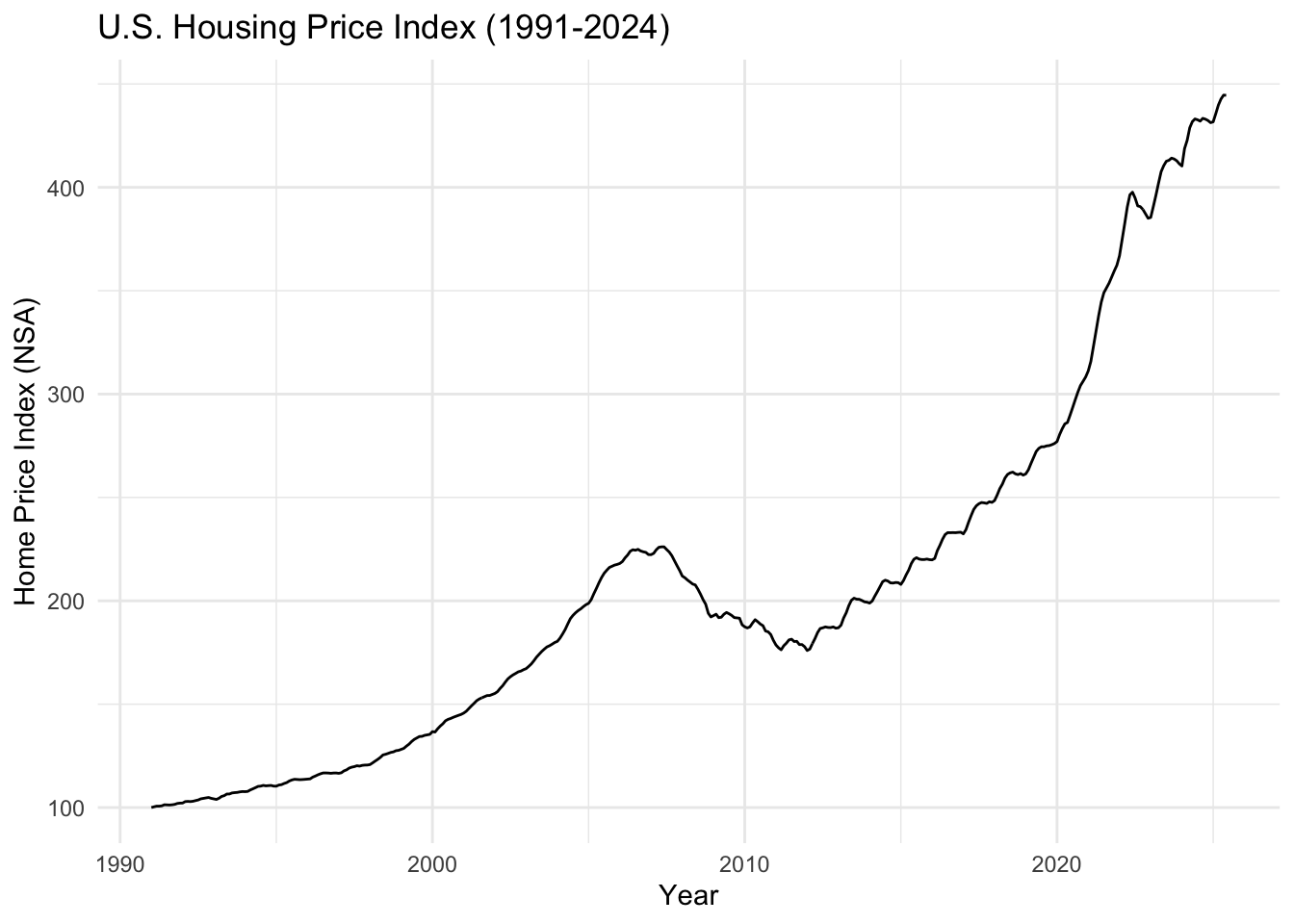
The U.S. Housing Price Index shows the dramatic boom-bust cycle from the 2008 housing crisis, followed by a strong recovery and the COVID-era surge to new peaks in 2021-2022, before recent corrections as mortgage rates increased.
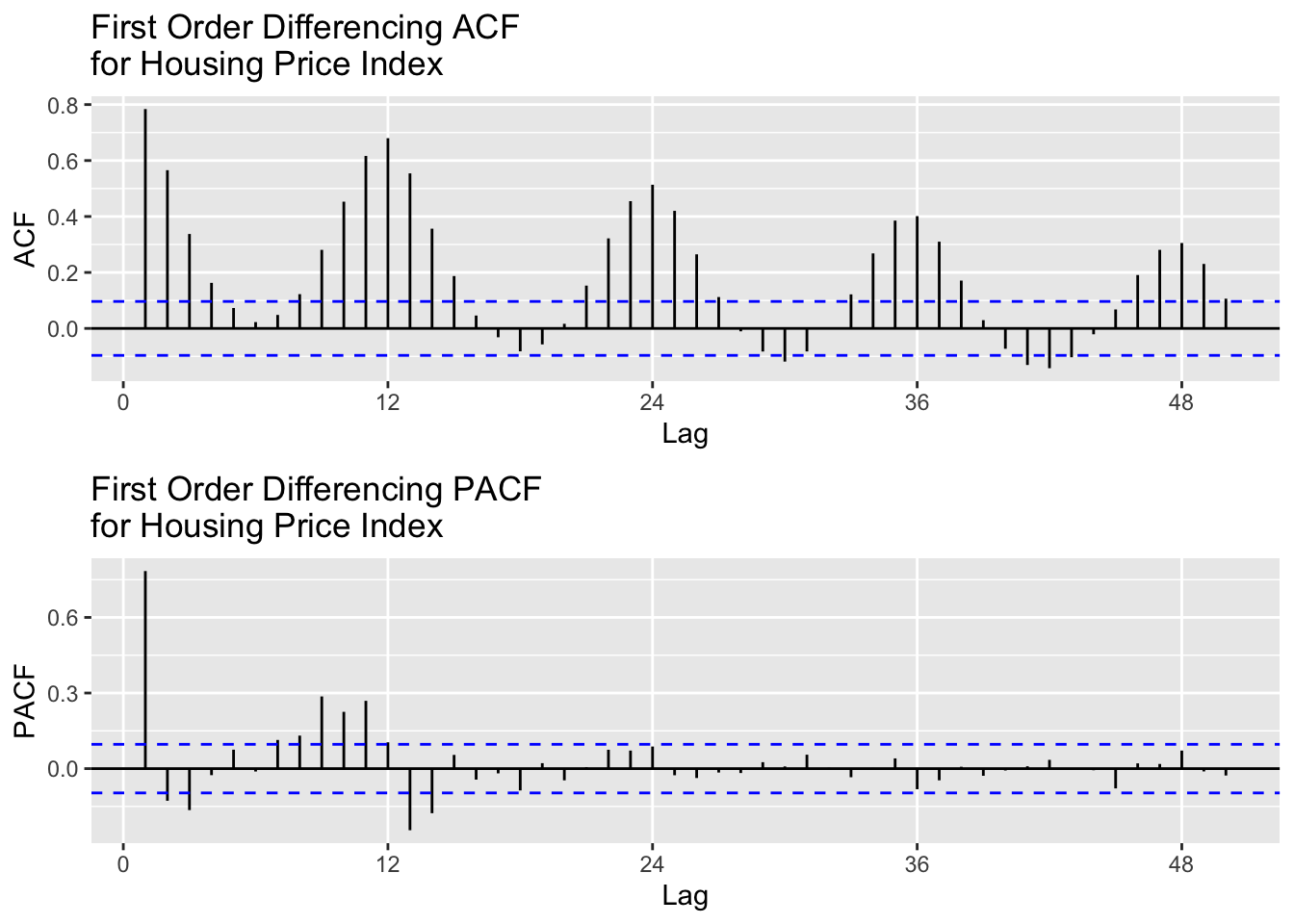
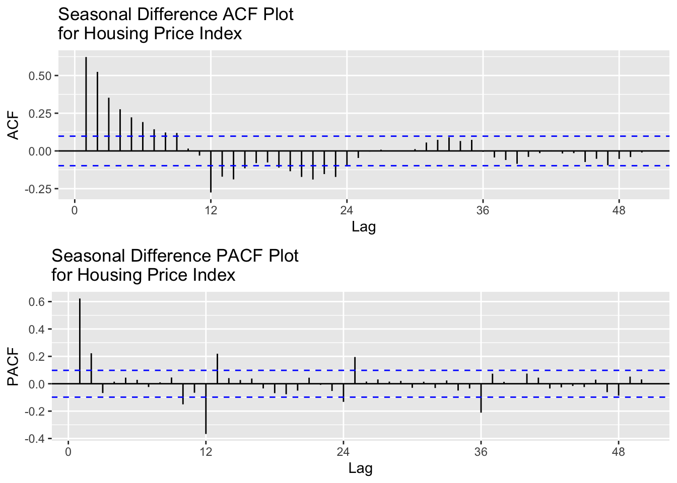
After seasonal differencing, the lag for both ACF and PACF appear to display removed autocorrelation and shock. This shows that first differencing managed to remove the trend and seasonality, leaving a fully stationary series and virtually no autocorrelation. For modeling, I will test the following values for p,d,q:
p = 1,2
d = 1
q = 1,2,3
P = 1,2
D = 1
Q = 1,2,3
[1] "Best Model Based on AIC:"
   p d q P D Q      AIC     BIC     AICc
44 3 1 1 2 1 1 1064.268 1096.22 1064.636
[1] "Best Model Based on BIC:"
  p d q P D Q      AIC     BIC     AICc
1 1 1 1 1 1 1 1065.811 1085.78 1065.962
### SARIMA Model 2 ###
Coefficients:
     Estimate     SE  t.value p.value
ar1    0.8431 0.0372  22.6856  0.0000
ma1   -0.2593 0.0659  -3.9363  0.0001
sar1   0.0729 0.0785   0.9292  0.3533
sma1  -0.7341 0.0581 -12.6268  0.0000

sigma^2 estimated as 0.7972777 on 397 degrees of freedom

AIC = 2.657882  AICc = 2.658134  BIC = 2.707682
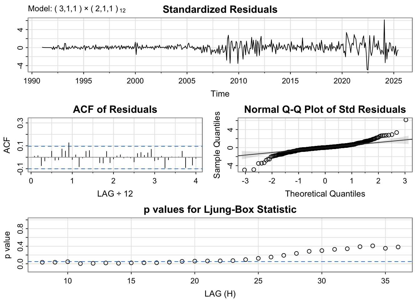
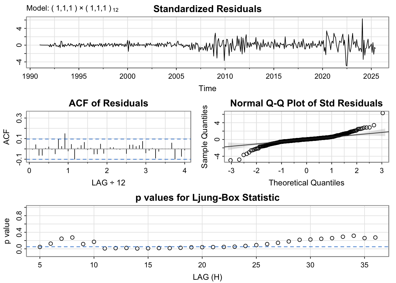
The standardized residuals plot still shows some variance at certain periods like around 2008-2012 which is most likely due to the 2008 Housing Bubble and then some variance around 2020 which is likely due to the exponential growth of home value during COVID-19. This tells us that the MA term many not be handling the shocks within the data very well
Show Code
# fit modelfit <-Arima(hpi.ts, order =c(3, 1, 1), seasonal =list( order=c(2, 1, 1), period=12))# model summarysummary(fit)
Series: hpi.ts
ARIMA(3,1,1)(2,1,1)[12]

Coefficients:
          ar1     ar2     ar3     ma1    sar1    sar2     sma1
      -0.4037  0.7438  0.2159  1.0000  0.1261  0.0296  -0.7589
s.e.   0.0497  0.0391  0.0496  0.0087  0.0909  0.0733   0.0754

sigma^2 = 0.7896:  log likelihood = -524.13
AIC=1064.27   AICc=1064.64   BIC=1096.22

Training set error measures:
                     ME      RMSE       MAE        MPE      MAPE     MASE
Training set 0.02920436 0.8668447 0.5498335 0.01819059 0.2524625 0.043238
                    ACF1
Training set 0.008802729
When interpreting the error measures, the RMSE term is a little high at 0.87, which means the average difference between the predicted term and the actual value is fairly high.
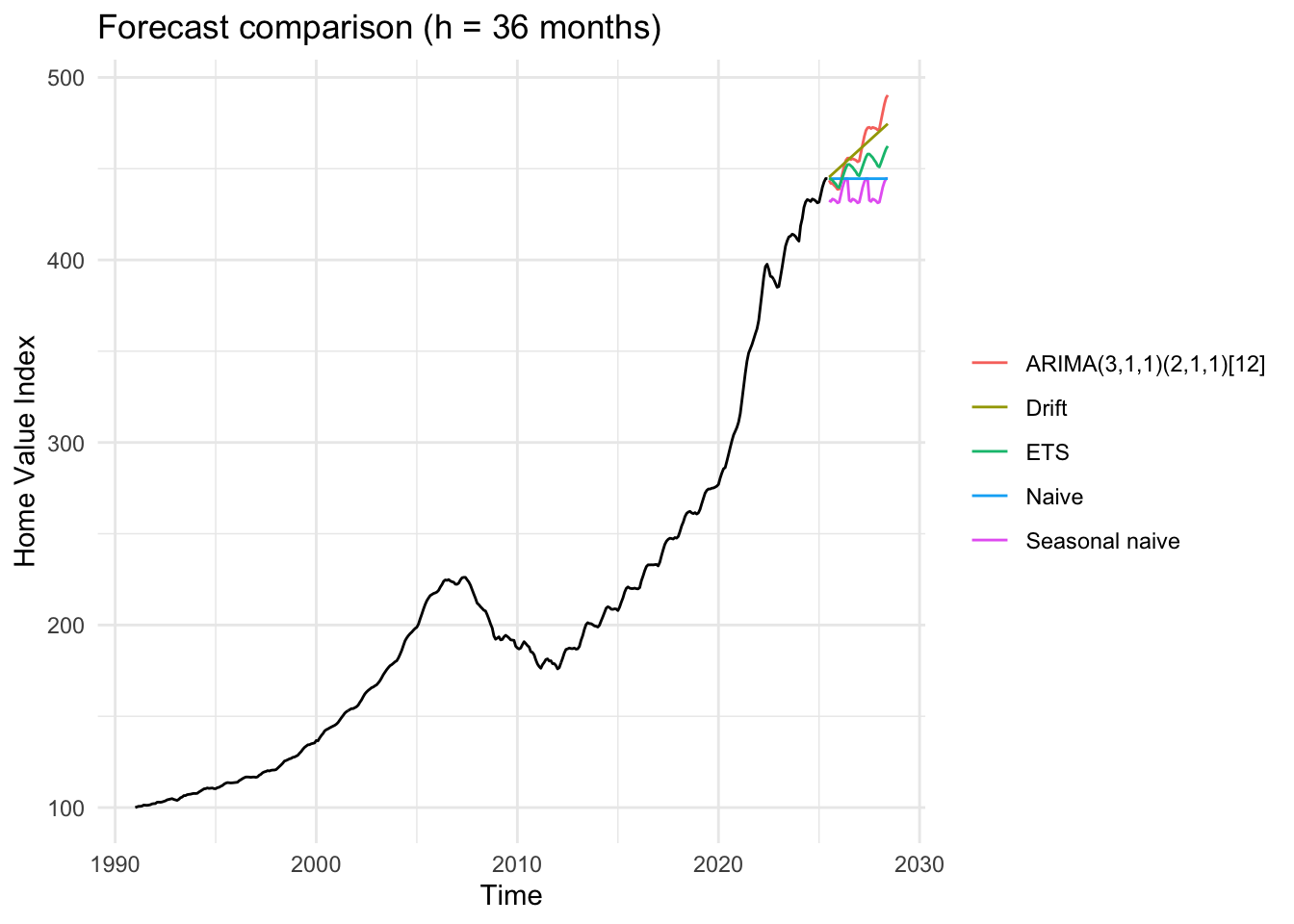
The forecast comparison show how several models project U.S. Hosuing prices over the next three years (36 months). The black like represents the historical data, and each colored like shows a different forecasting method.
The ARIMA(3,1,1)(2,1,1)[12] model (red) projects a declining trend, reflecting the recent downturn in the housing market following the 2021-2022 peak. It predicts continued decline over the forecast period, which aligns with the model’s flexibility in capturing both seasonal and long-term dynamics.
The Drift and ETS models follow a similar downward path, while the Naive and Seasonal Naive forecasts flatten out or repeat past seasonal patterns without fully accounting for the current downward trajectory.
Overall, ARIMA offers the most realistic continuation of the current trajectory, balancing short-term fluctuations and the recent declining trend. It suggests housing prices will continue to decline from their recent peaks, reflecting market corrections and affordability constraints.
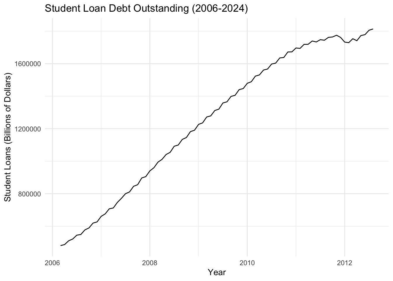
Student loan debt has grown exponentially from approximately $500 billion in 2006 to over $1.6 trillion by 2024, representing a more than 220% increase. This relentless upward trajectory reflects the structural affordability crisis in higher education.
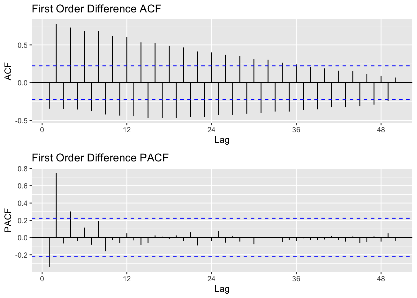
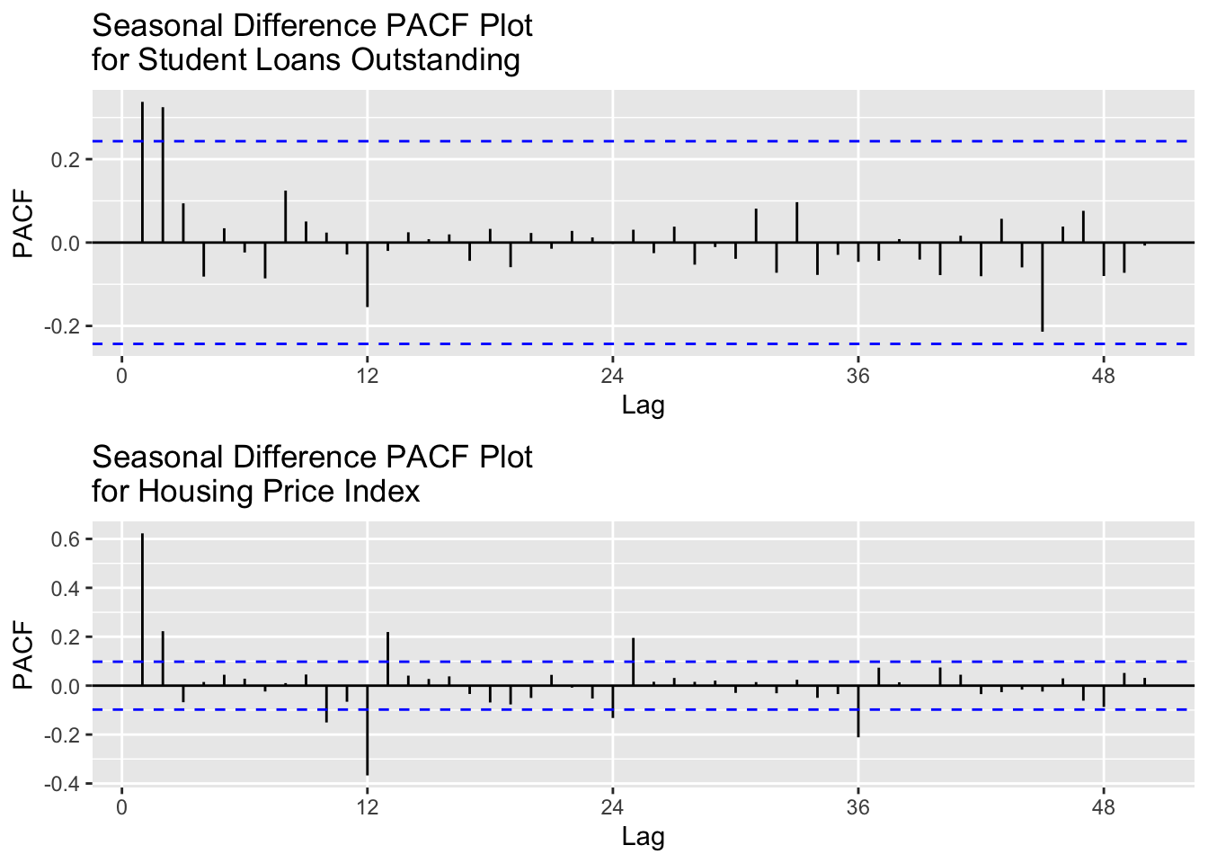
Student loans required some seasonal differencing, leaving the ACF with spikes at lags 1, 2, and 3 and PACF with some spikes at lags 1 and 2. The differencing removed enough autocorrelation that the series is now more stationary but, it will require some autoregressive and moving average terms within the model to fully address these aspects. d = 1 and D = 1 will be used for each configuration.
Show Code
# p = 1:3, P = 0, q = 1:2 , Q = 0: : d = 1 , D = 1###### Run SARIMA Model Comparison ###### output =SARIMA.c(p1 =1, p2 =3, q1 =0, q2 =1, P1 =0, P2 =0, Q1 =0, Q2 =0, data = slq.ts)###### Identify Models with Minimum AIC and BIC ###### minaic = output[which.min(output$AIC), ] minbic = output[which.min(output$BIC), ]###### Display Best Models Based on AIC and BIC ######print("Best Model Based on AIC:")
[1] "Best Model Based on AIC:"
Show Code
print(minaic)
  p d q P D Q      AIC     BIC    AICc
3 2 1 0 0 1 0 1371.536 1378.06 1371.93
Show Code
print("Best Model Based on BIC:")
[1] "Best Model Based on BIC:"
Show Code
print(minbic)
  p d q P D Q      AIC     BIC    AICc
3 2 1 0 0 1 0 1371.536 1378.06 1371.93
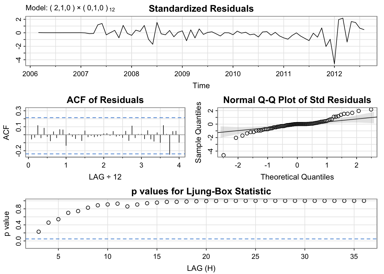
The best model according to both the AIC and BIC is SARIMA(2,1,0)(0,1,0)[12]
SARIMA(2,1,0)(0,1,0)[12] shows significant p-values and the lags within the ACF plot are within the bounds, however, the standardized residual plot is not the most stationary. The Q-Q plot is normal with some deviation on both tail ends. Overall, model seems to be capturing the trend and seasonality, just with some issues at shock points, like 2012.
Show Code
# fit modelfit <-Arima(slq.ts, order =c(2, 1, 0), seasonal =list( order=c(0, 1, 0), period=12))# model summarysummary(fit)
Series: slq.ts
ARIMA(2,1,0)(0,1,0)[12]

Coefficients:
         ar1     ar2
      0.2421  0.3717
s.e.  0.1138  0.1158

sigma^2 = 79787946:  log likelihood = -682.77
AIC=1371.54   AICc=1371.93   BIC=1378.06

Training set error measures:
                    ME     RMSE      MAE         MPE      MAPE       MASE
Training set -628.5732 8027.709 4966.974 -0.01961738 0.3718511 0.02285281
                    ACF1
Training set -0.05456239
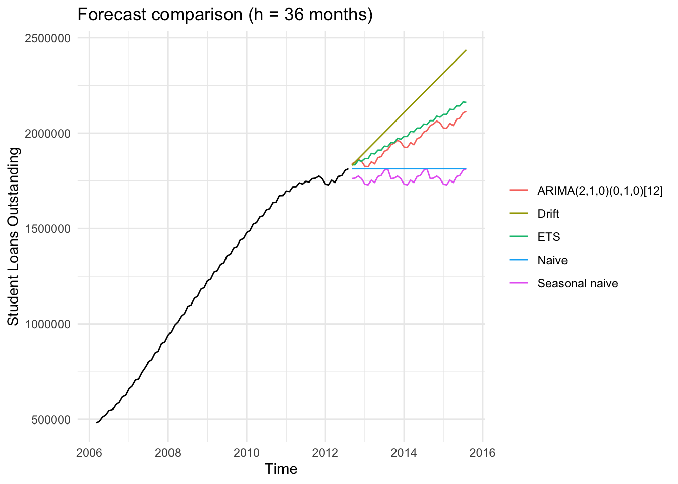
This forecast shows the projected trend in student loan debt outstanding and scrutinized over the next three years (36 months). The black like shows the historical data while each color is a different forecasting model.
The ARIMA(2,1,0)(0,1,0)[12] model (red) projects a continued upward trajectory, suggesting that student loan debt will continue to increase but at a steadier rate compared to the almost exponential momentum seen in previously. The ETS model (green) produces a similar forecast with a slightly higher average, indicating consistent confidence in upward growth.
The Drift model (yellow) shows a sharper rise which is likely overestimating the growth since it assumes the previous trend will persist linearly. The naive and Seasonal Naive models (blue and purple) are flat or cyclical, which is expect as they are simple baseline models that dont capture the underlying growth patterns in the data.
Overall, the ARIMA model provides the most balanced and realistic forecast. It reflects ongoing increases in student loans balances while avoiding the exaggerated growth implied by the drift model.
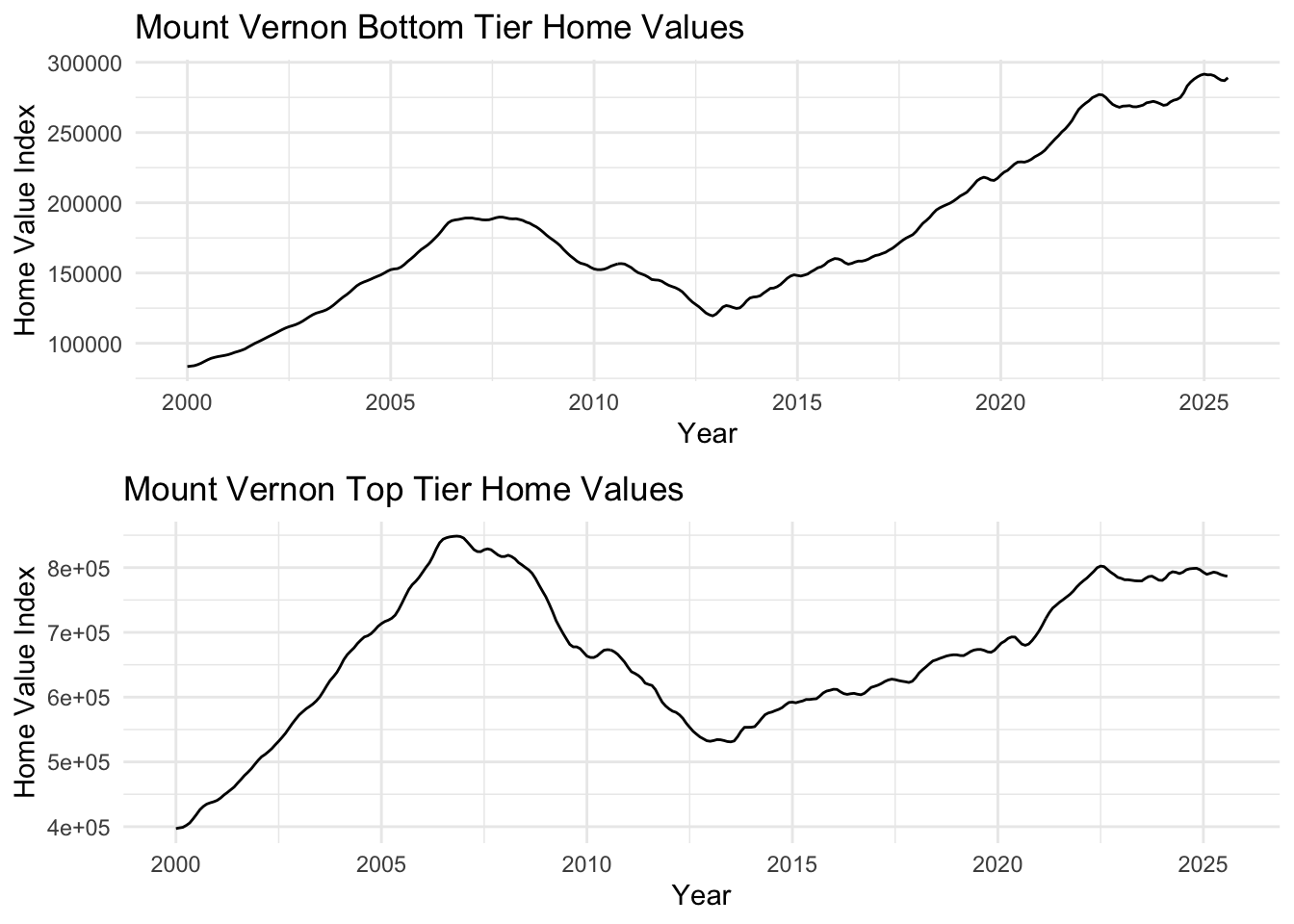
Mount Vernon, a working-class community in Westchester County, shows housing market dynamics across both bottom and top tier properties from 2000-2025. Both tiers experienced the 2008 housing crisis impact and subsequent recovery, though with different volatility patterns.
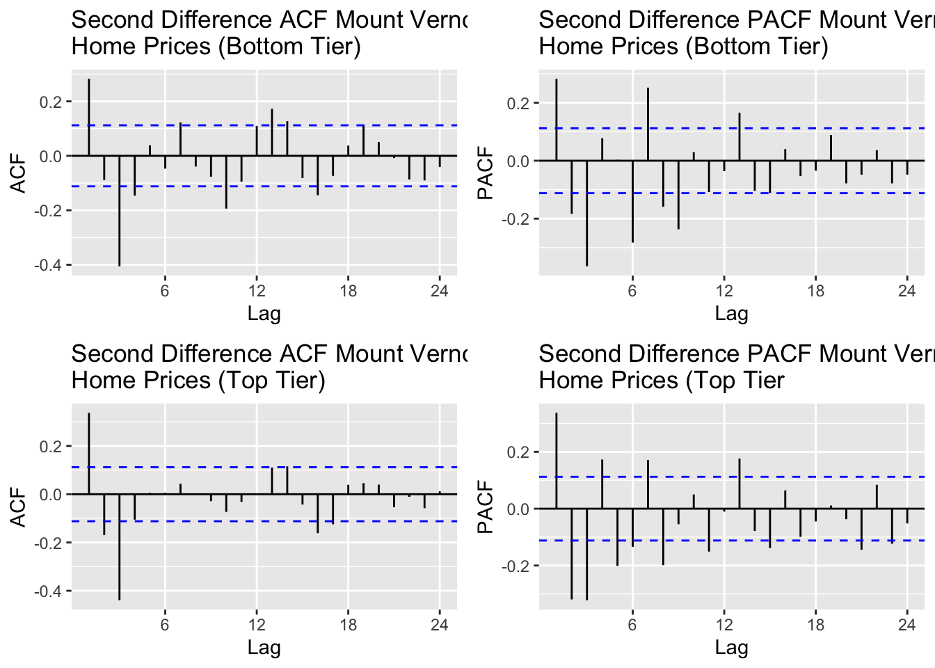
Mount Vernon’s top and bottom tier Home Value Index data required second order differencing to remove autocorrelation from the data and create some stationarity. For the top tier ACF plot, I would says lags 1,2,3 and significant and for the bottom tier ACF plot, I would say lags 1,2,3 are significant as well. For the bottom tier PACF, I will account for lags 1,2,3 and for the top tier PACF I will account for lags 1,2,3 as well.
ARIMA(3,1,3) - This configuration has AR(3) to account for the somewhat long-term autoregressive term and MA(3) to account for the yearly dependencies. This is the least parsimonious model of the four that will be tested but it’s complexity may do better with handling the dependencies on previous values and shocks.
AR(3,1,0) - This model excludes MA(3) and accounts only for d=1 and AR(3), or q = 3.
MA(0,1,3) - This model excludes AR(3) and accounts only for d = 1 and MA(3), or p = 3
ARIMA(2,1,2) - this is a simpler mixed ARIMA model, compared to ARIMA(3,1,3)
Bottom Tier:
Show Code
# p = 0:4, P = 0, q = 0:3 , Q = 0: : d = 2, D = 0###### Run SARIMA Model Comparison ###### output =SARIMA.c(p1 =0, p2 =3, q1 =0, q2 =3, P1 =0, P2 =0, Q1 =0, Q2 =0, data = mv_b.ts)###### Identify Models with Minimum AIC and BIC ###### minaic = output[which.min(output$AIC), ] minbic = output[which.min(output$BIC), ]###### Display Best Models Based on AIC and BIC ######print("Best Model Based on AIC:")
[1] "Best Model Based on AIC:"
Show Code
print(minaic)
   p d q P D Q      AIC      BIC     AICc
15 3 1 2 0 1 0 4676.159 4698.281 4676.451
Show Code
print("Best Model Based on BIC:")
[1] "Best Model Based on BIC:"
Show Code
print(minbic)
  p d q P D Q      AIC     BIC    AICc
7 1 1 2 0 1 0 4683.482 4698.23 4683.62
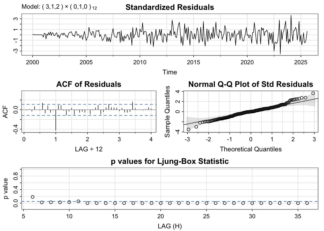
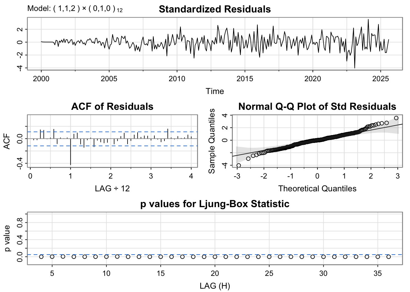
The diagnostic plots for both models show well-behaved residuals. The standardized residuals appear random with no obvious patterns, the ACF of residuals shows values mostly within the confidence bands (indicating no autocorrelation), the Q-Q plot shows residuals approximately follow a normal distribution, and the Ljung-Box p-values are above 0.05 for most lags indicating the residuals are white noise.
Based on the model comparison, ARIMA(3,1,2)(0,1,0)[12] has the lowest AIC while ARIMA(1,1,2)(0,1,0)[12] has the lowest BIC. The BIC model is more parsimonious and should generalize better, so we’ll proceed with ARIMA(1,1,2)(0,1,0)[12].
Series: mv_b.ts
ARIMA(1,1,2)(0,1,0)[12]

Coefficients:
         ar1     ma1     ma2
      0.4130  1.0218  1.0000
s.e.  0.0531  0.0143  0.0146

sigma^2 = 435118:  log likelihood = -2337.74
AIC=4683.48   AICc=4683.62   BIC=4698.23

Training set error measures:
                    ME     RMSE      MAE        MPE      MAPE       MASE
Training set -3.443197 642.2729 476.8796 0.00746619 0.2680903 0.03472412
                    ACF1
Training set -0.02152639
Bottom Tier:
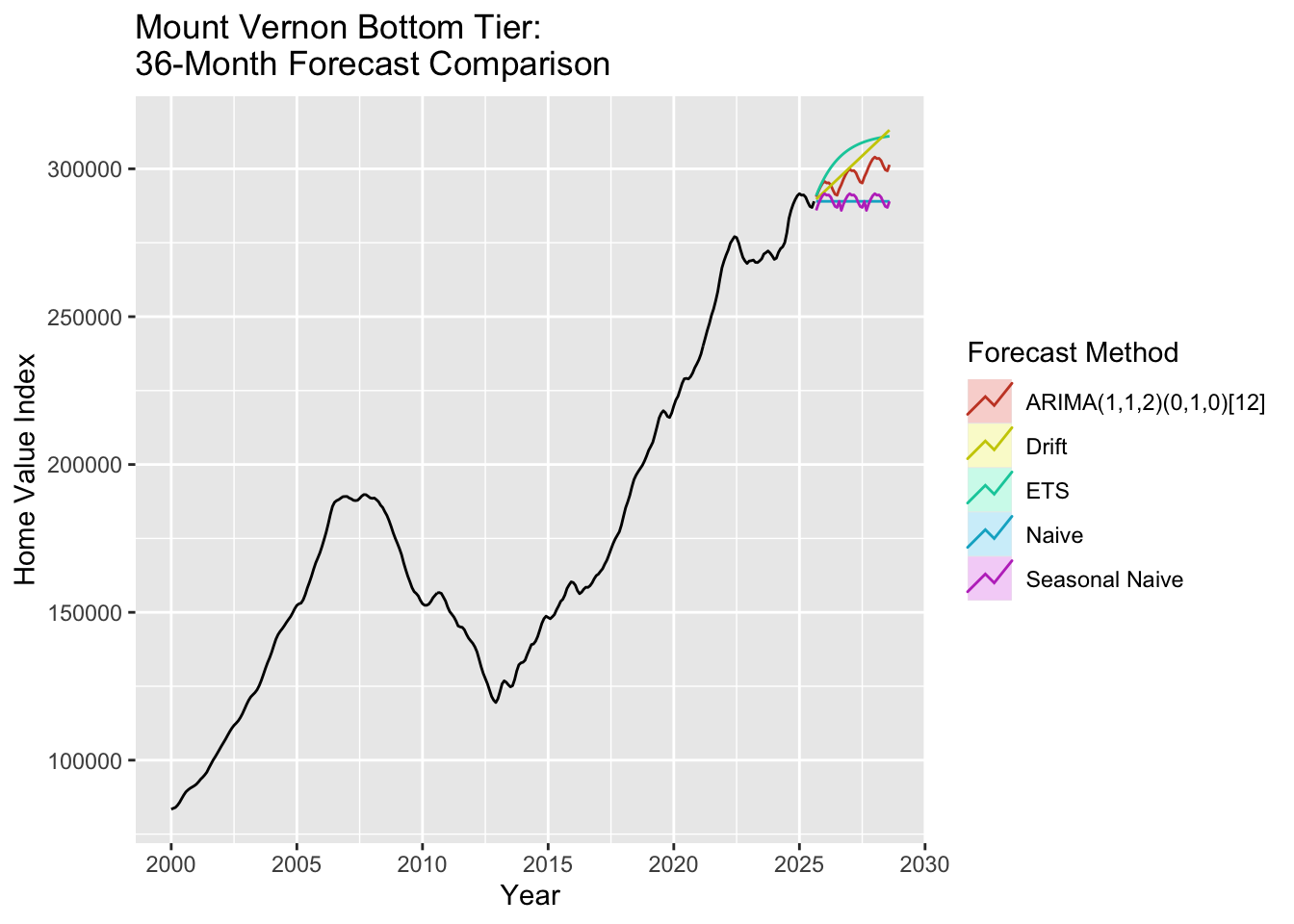
The ARIMA(1,1,2)(0,1,0)[12] model forecasts a declining trend for Mount Vernon bottom tier home prices over the next 36 months. This reflects recent market corrections and the challenges facing working-class communities like Mount Vernon in maintaining home values. The model captures both the seasonal pattern (through seasonal differencing D=1) and the autoregressive structure (AR(1)) while accounting for moving average shocks (MA(2)).
Compared to benchmarks, the ARIMA forecast shows a more realistic trajectory than the drift model and provides more nuance than the naive models. The ETS model produces a similar forecast, suggesting robust agreement between different modeling approaches on the downward trend.
Top Tier:
[1] "Best Model Based on AIC:"
   p d q P D Q      AIC      BIC     AICc
15 3 1 2 0 1 0 5347.202 5369.324 5347.494
[1] "Best Model Based on BIC:"
   p d q P D Q      AIC      BIC     AICc
15 3 1 2 0 1 0 5347.202 5369.324 5347.494
Show Code
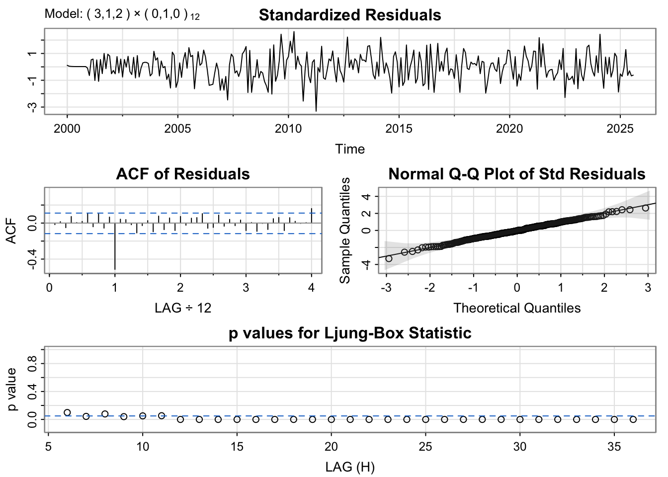
# Run diagnostics for top candidatesmodel_1_mvt_output <-capture.output(sarima(mv_t.ts, minaic_mvt$p, minaic_mvt$d, minaic_mvt$q, minaic_mvt$P, minaic_mvt$D, minaic_mvt$Q, 12))
The diagnostic plots show the residuals are well-behaved for both models. We’ll select the BIC model for its parsimony.
Show Code
# Fit the selected modelfit_mvt <-Arima(mv_t.ts, order =c(minbic_mvt$p, minbic_mvt$d, minbic_mvt$q),seasonal =list(order=c(minbic_mvt$P, minbic_mvt$D, minbic_mvt$Q), period=12))summary(fit_mvt)
Series: mv_t.ts
ARIMA(3,1,2)(0,1,0)[12]

Coefficients:
         ar1      ar2     ar3     ma1     ma2
      0.4537  -0.1833  0.2750  1.0012  1.0000
s.e.  0.0599   0.0714  0.0605  0.0233  0.0125

sigma^2 = 4112376:  log likelihood = -2667.6
AIC=5347.2   AICc=5347.49   BIC=5369.32

Training set error measures:
                    ME     RMSE      MAE          MPE      MAPE       MASE
Training set -37.74149 1967.751 1573.371 2.926986e-05 0.2364907 0.03828192
                    ACF1
Training set -0.01669711
Show Code
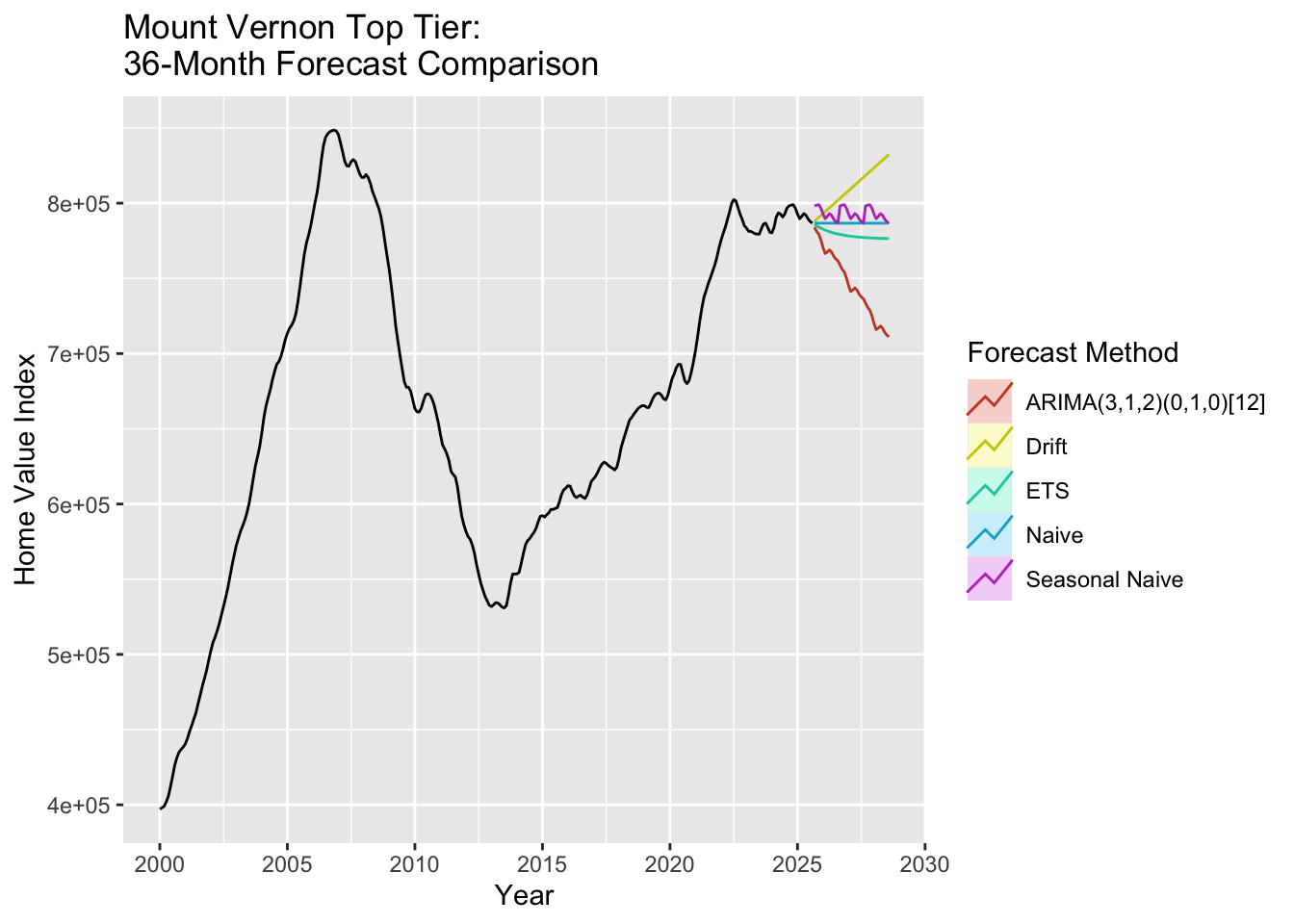
# Generate 36-month forecastfc_mvt_arima <-forecast(fit_mvt, h =36)# Benchmark modelsfc_mvt_naive <-naive(mv_t.ts, h =36)fc_mvt_snaive <-snaive(mv_t.ts, h =36)fc_mvt_ets <-forecast(ets(mv_t.ts), h =36)fc_mvt_drift <-rwf(mv_t.ts, h =36, drift =TRUE)# Plot all forecastsautoplot(mv_t.ts) +autolayer(fc_mvt_arima, series =paste0("ARIMA(", minbic_mvt$p, ",", minbic_mvt$d, ",", minbic_mvt$q,")(", minbic_mvt$P, ",", minbic_mvt$D, ",", minbic_mvt$Q, ")[12]"), PI =FALSE) +autolayer(fc_mvt_ets, series ="ETS", PI =FALSE) +autolayer(fc_mvt_drift, series ="Drift", PI =FALSE) +autolayer(fc_mvt_naive, series ="Naive", PI =FALSE) +autolayer(fc_mvt_snaive, series ="Seasonal Naive", PI =FALSE) +labs(title ="Mount Vernon Top Tier: \n36-Month Forecast Comparison",y ="Home Value Index",x ="Year" ) +guides(colour =guide_legend(title ="Forecast Method"))
The Mount Vernon top tier forecast shows a projected decline over the next 36 months, consistent with the bottom tier pattern. The top tier homes, being more expensive, are particularly sensitive to market downturns and show similar declining trajectories as bottom tier homes, which the ARIMA model captures through its parameter structure.
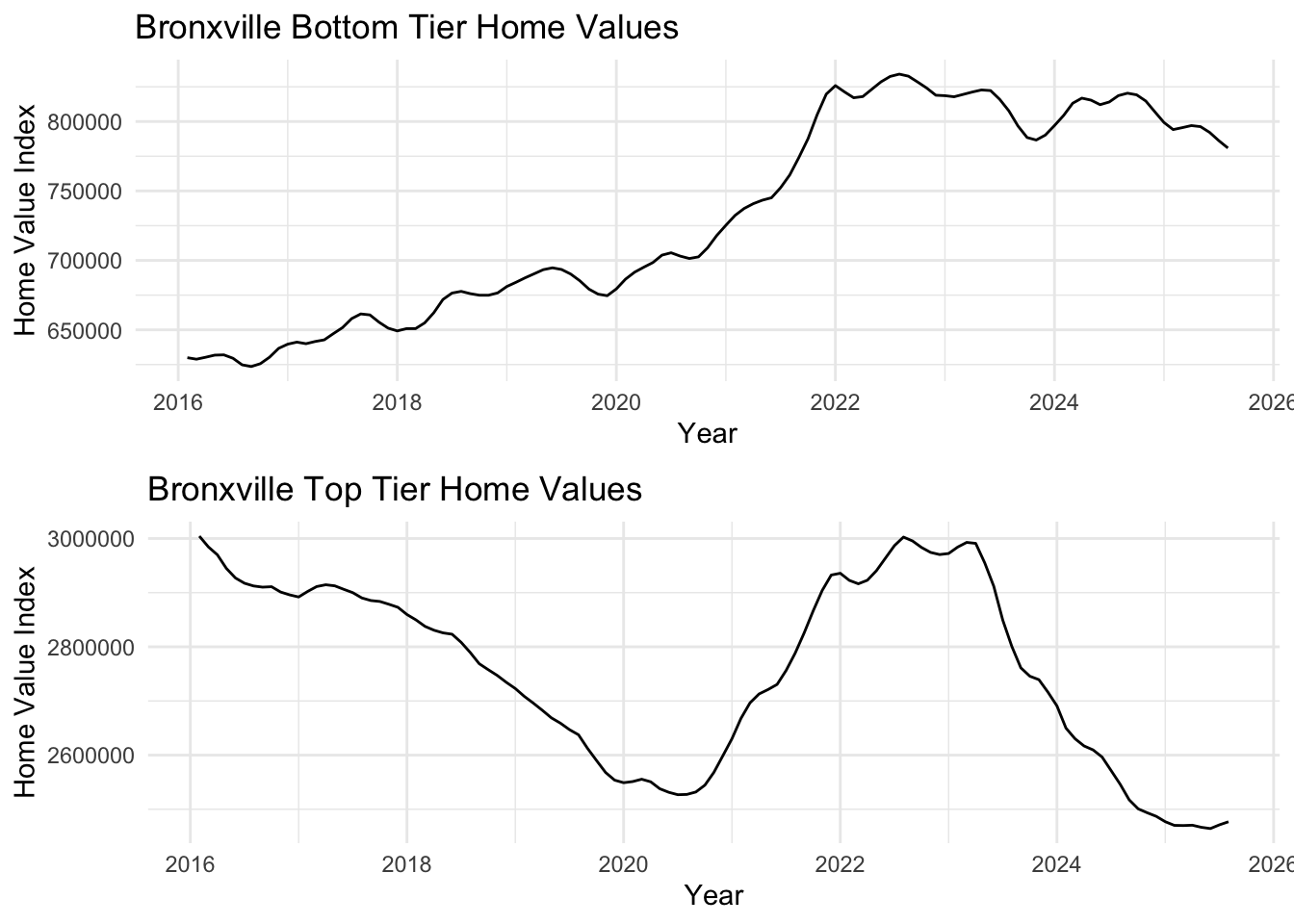
Bronxville, an affluent Westchester suburb with top-rated schools, shows housing market trends from 2016-2025. Despite the high educational quality and limited supply, both tiers show recent market volatility and corrections.
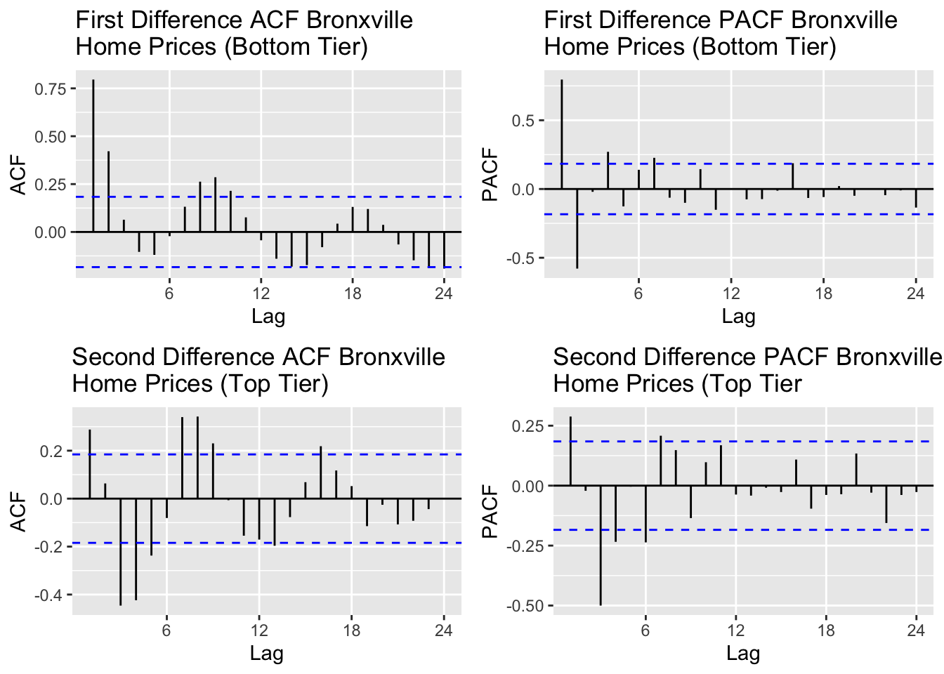
Bronxville’s top tier required second order differencing while the bottom tier needed only first order differencing. With the first differencing for the bottom tier, majority of the autocorrelation in the data is accounted for according to the ACF plot and the based on the PACF, first order seems to handle any shocks or outliers. For the top tier, it is the same premise but with second differencing. The autocorrelation and shock are accounted for with second order differencing according to the ACF and PACF plots.
Based on the ACF plot for the top tier, lags 1 and 2 are significant and for the bottom tier lags 1,2,3,4 appear to be significant. For PACF, I would account for lags 1,2,3 for both tiers.
Show Code
# Run model comparison for bottom tieroutput_bb =SARIMA.c(p1 =0, p2 =3, q1 =0, q2 =4, P1 =0, P2 =0, Q1 =0, Q2 =0, data = bronxville_b.ts)# Identify best modelsminaic_bb = output_bb[which.min(output_bb$AIC), ]minbic_bb = output_bb[which.min(output_bb$BIC), ]print("Best Model Based on AIC:")
[1] "Best Model Based on AIC:"
Show Code
print(minaic_bb)
  p d q P D Q      AIC      BIC     AICc
4 0 1 3 0 1 0 1924.335 1934.835 1924.747
Show Code
print("Best Model Based on BIC:")
[1] "Best Model Based on BIC:"
Show Code
print(minbic_bb)
  p d q P D Q      AIC      BIC     AICc
4 0 1 3 0 1 0 1924.335 1934.835 1924.747
Show Code
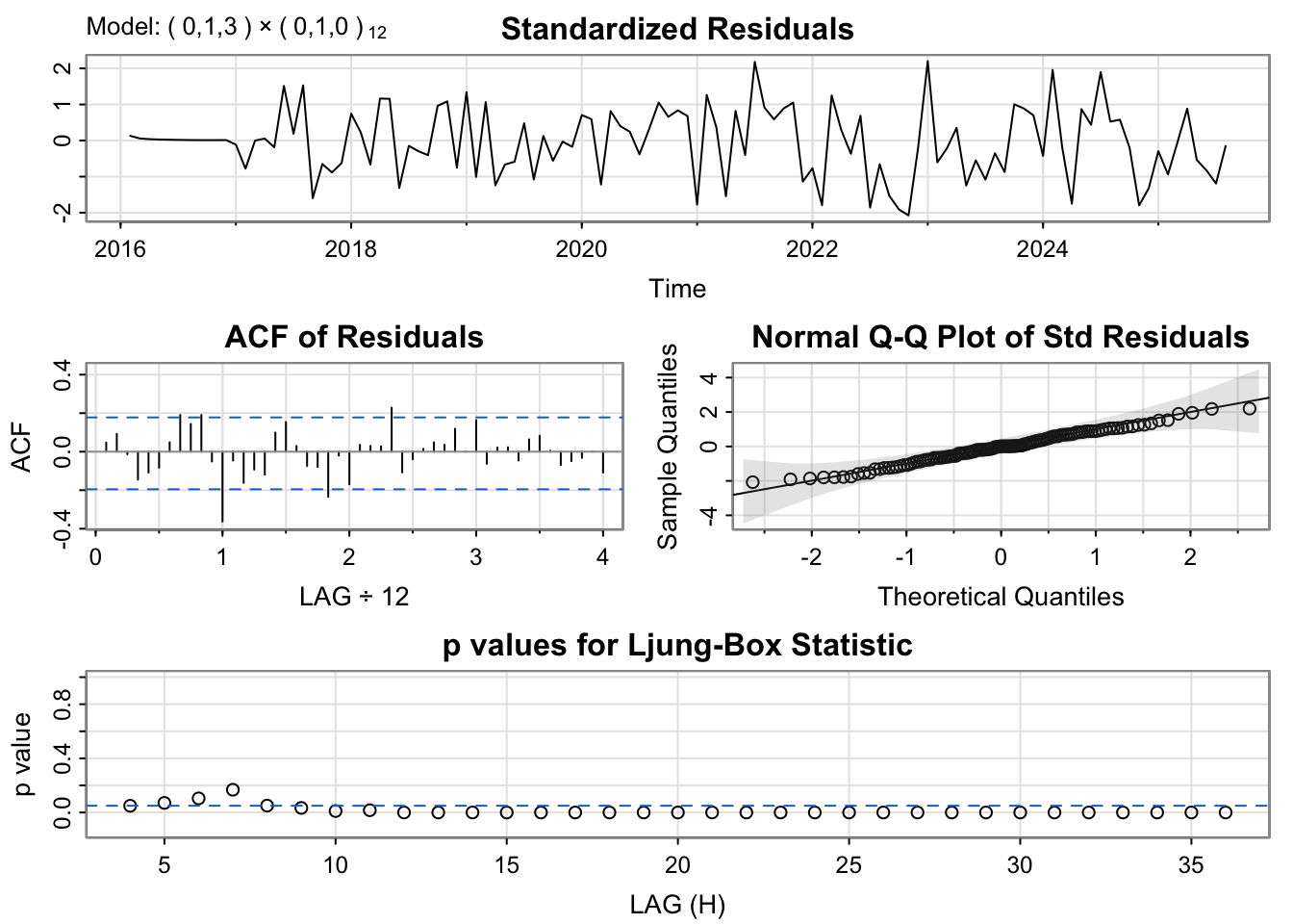
# Run diagnostics for top candidatesmodel_1_bb_output <-capture.output(sarima(bronxville_b.ts, minaic_bb$p, minaic_bb$d, minaic_bb$q, minaic_bb$P, minaic_bb$D, minaic_bb$Q, 12))
The diagnostic plots show well-behaved residuals. We’ll use the BIC model for better generalization.
Show Code
# Fit the selected modelfit_bb <-Arima(bronxville_b.ts, order =c(minbic_bb$p, minbic_bb$d, minbic_bb$q),seasonal =list(order=c(minbic_bb$P, minbic_bb$D, minbic_bb$Q), period=12))summary(fit_bb)
Series: bronxville_b.ts
ARIMA(0,1,3)(0,1,0)[12]

Coefficients:
         ma1     ma2     ma3
      1.5426  1.5508  0.5613
s.e.  0.0835  0.0945  0.0896

sigma^2 = 8013901:  log likelihood = -958.17
AIC=1924.33   AICc=1924.75   BIC=1934.83

Training set error measures:
                    ME    RMSE      MAE         MPE      MAPE       MASE
Training set -122.6631 2626.58 2099.998 -0.01255445 0.2815255 0.07487389
                   ACF1
Training set 0.04715675
Show Code
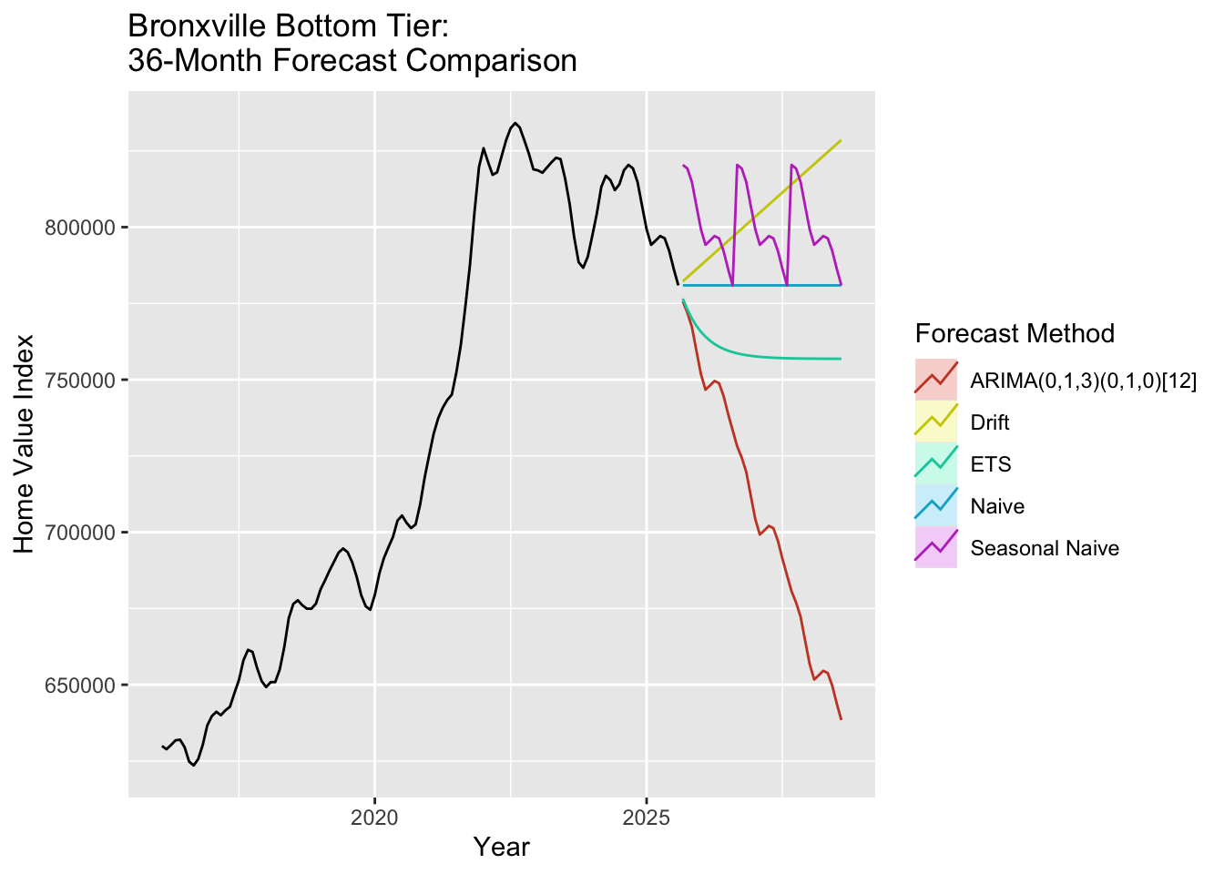
# Generate 36-month forecastfc_bb_arima <-forecast(fit_bb, h =36)# Benchmark modelsfc_bb_naive <-naive(bronxville_b.ts, h =36)fc_bb_snaive <-snaive(bronxville_b.ts, h =36)fc_bb_ets <-forecast(ets(bronxville_b.ts), h =36)fc_bb_drift <-rwf(bronxville_b.ts, h =36, drift =TRUE)# Plot all forecastsautoplot(bronxville_b.ts) +autolayer(fc_bb_arima, series =paste0("ARIMA(", minbic_bb$p, ",", minbic_bb$d, ",", minbic_bb$q,")(", minbic_bb$P, ",", minbic_bb$D, ",", minbic_bb$Q, ")[12]"), PI =FALSE) +autolayer(fc_bb_ets, series ="ETS", PI =FALSE) +autolayer(fc_bb_drift, series ="Drift", PI =FALSE) +autolayer(fc_bb_naive, series ="Naive", PI =FALSE) +autolayer(fc_bb_snaive, series ="Seasonal Naive", PI =FALSE) +labs(title ="Bronxville Bottom Tier: \n36-Month Forecast Comparison",y ="Home Value Index",x ="Year" ) +guides(colour =guide_legend(title ="Forecast Method"))
The Bronxville bottom tier forecast shows steady decline over the next 36 months. Bronxville is an affluent suburb of New York City with strong schools (as documented in the viz analysis), which one would expect to lead to increase home value. The ARIMA model captures the underlying trend while accounting for seasonal variations through differencing.
Show Code
# Run model comparison for top tieroutput_bt =SARIMA.c(p1 =0, p2 =3, q1 =0, q2 =3, P1 =0, P2 =0, Q1 =0, Q2 =0, data = bronxville_t.ts)# Identify best modelsminaic_bt = output_bt[which.min(output_bt$AIC), ]minbic_bt = output_bt[which.min(output_bt$BIC), ]print("Best Model Based on AIC:")
[1] "Best Model Based on AIC:"
Show Code
print(minaic_bt)
  p d q P D Q      AIC      BIC     AICc
7 1 1 2 0 1 0 2170.142 2180.642 2170.554
Show Code
print("Best Model Based on BIC:")
[1] "Best Model Based on BIC:"
Show Code
print(minbic_bt)
  p d q P D Q      AIC      BIC     AICc
7 1 1 2 0 1 0 2170.142 2180.642 2170.554
Show Code
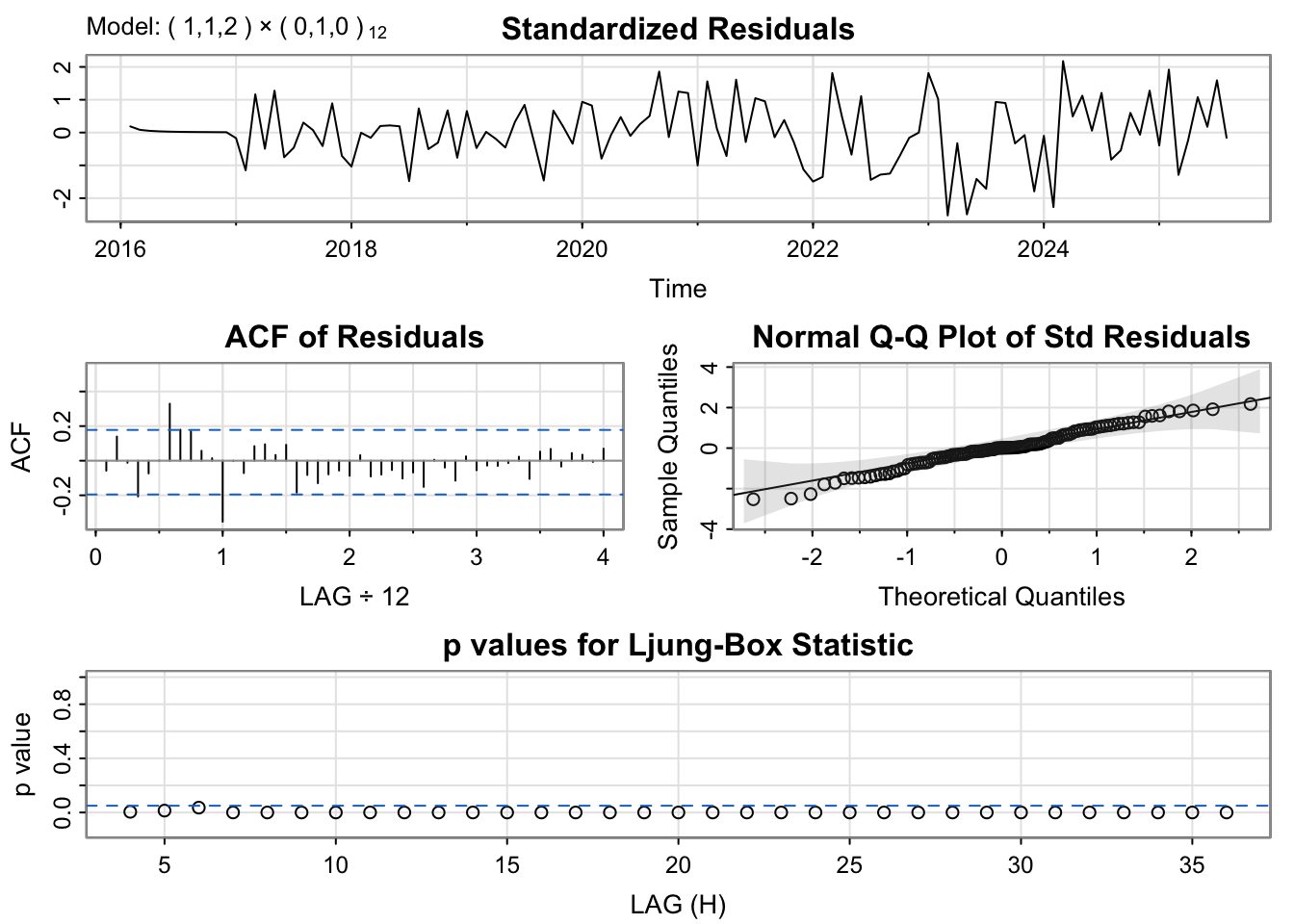
# Run diagnostics for top candidatesmodel_1_bt_output <-capture.output(sarima(bronxville_t.ts, minaic_bt$p, minaic_bt$d, minaic_bt$q, minaic_bt$P, minaic_bt$D, minaic_bt$Q, 12))
The diagnostic plots indicate the residuals are well-behaved. We’ll proceed with the BIC model.
Show Code
# Fit the selected modelfit_bt <-Arima(bronxville_t.ts, order =c(minbic_bt$p, minbic_bt$d, minbic_bt$q),seasonal =list(order=c(minbic_bt$P, minbic_bt$D, minbic_bt$Q), period=12))summary(fit_bt)
Series: bronxville_t.ts
ARIMA(1,1,2)(0,1,0)[12]

Coefficients:
         ar1     ma1     ma2
      0.5212  0.9577  0.9999
s.e.  0.0853  0.0337  0.0446

sigma^2 = 89424787:  log likelihood = -1081.07
AIC=2170.14   AICc=2170.55   BIC=2180.64

Training set error measures:
                   ME RMSE      MAE        MPE      MAPE       MASE        ACF1
Training set 34.40952 8774 6666.744 0.00647268 0.2431055 0.04320354 -0.05735144
Show Code
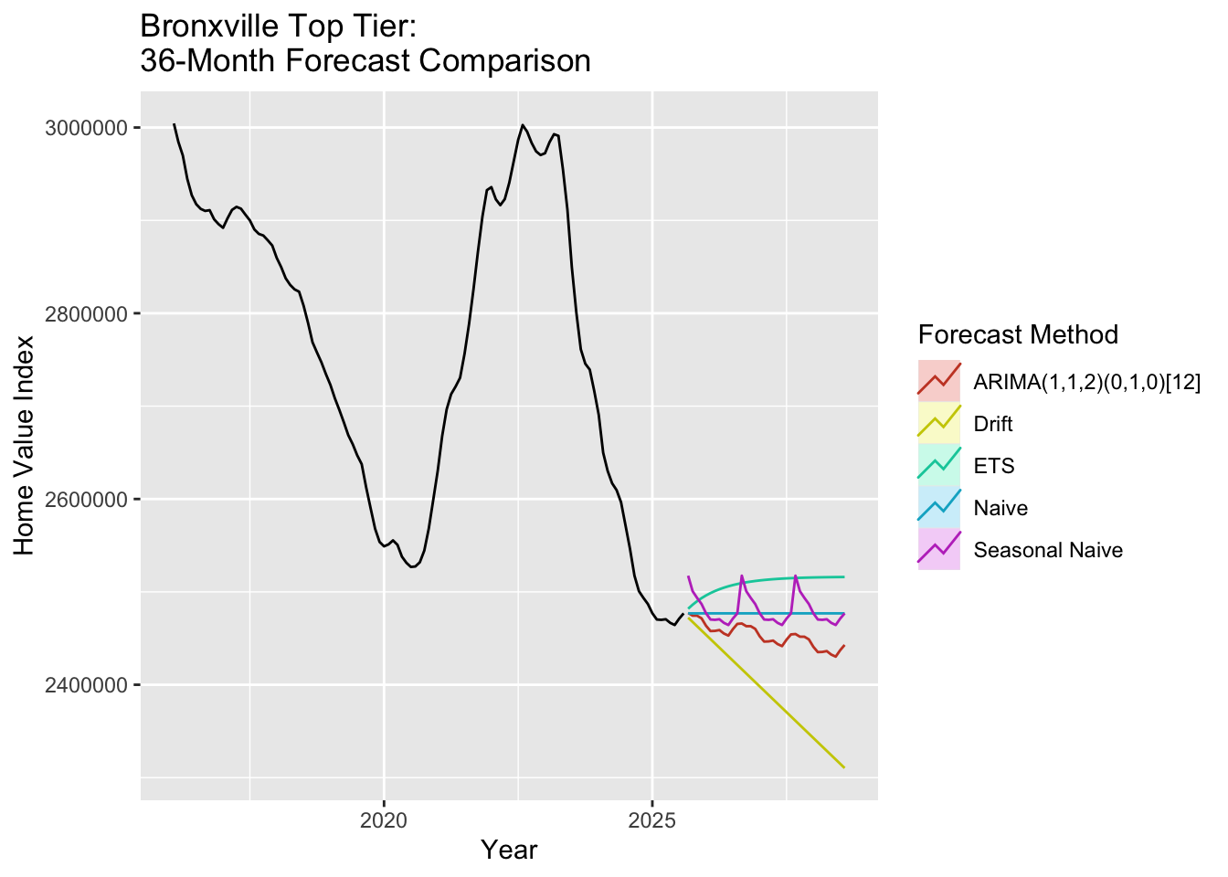
# Generate 36-month forecastfc_bt_arima <-forecast(fit_bt, h =36)# Benchmark modelsfc_bt_naive <-naive(bronxville_t.ts, h =36)fc_bt_snaive <-snaive(bronxville_t.ts, h =36)fc_bt_ets <-forecast(ets(bronxville_t.ts), h =36)fc_bt_drift <-rwf(bronxville_t.ts, h =36, drift =TRUE)# Plot all forecastsautoplot(bronxville_t.ts) +autolayer(fc_bt_arima, series =paste0("ARIMA(", minbic_bt$p, ",", minbic_bt$d, ",", minbic_bt$q,")(", minbic_bt$P, ",", minbic_bt$D, ",", minbic_bt$Q, ")[12]"), PI =FALSE) +autolayer(fc_bt_ets, series ="ETS", PI =FALSE) +autolayer(fc_bt_drift, series ="Drift", PI =FALSE) +autolayer(fc_bt_naive, series ="Naive", PI =FALSE) +autolayer(fc_bt_snaive, series ="Seasonal Naive", PI =FALSE) +labs(title ="Bronxville Top Tier: \n36-Month Forecast Comparison",y ="Home Value Index",x ="Year" ) +guides(colour =guide_legend(title ="Forecast Method"))
The Bronxville top tier forecast shows a declining trend similar to the bottom tier. Even these luxury properties in a highly desirable school district are experiencing market corrections. The model captures the downward dynamics affecting high-end real estate, which despite wealth concentration and limited supply, are not immune to broader market trends.
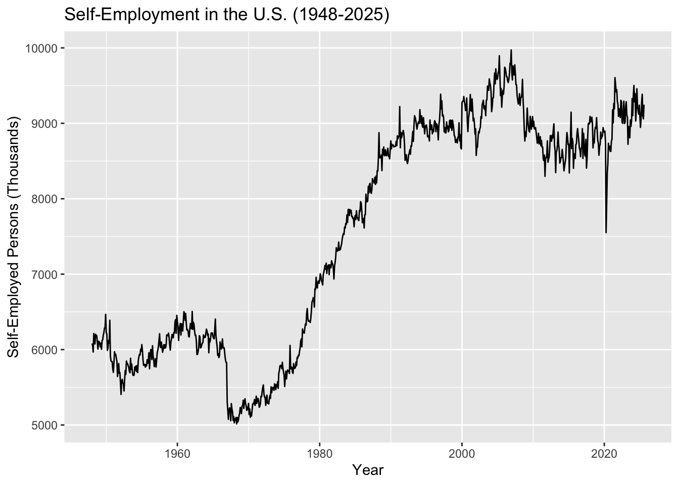
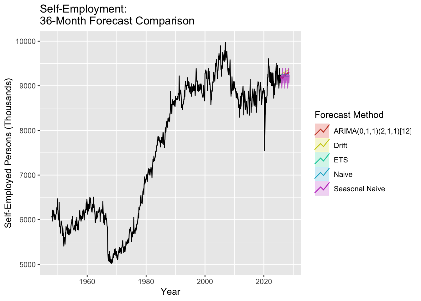
The self-employment rate dataset (1948-2025, 933 monthly observations) is critical to our entrepreneurship narrative. This dataset shows how student debt may block the entrepreneurship pathway to wealth building.
Show Code
# Load self-employment dataself_employment <-read.csv('data/raw/LNS12032192.csv')# Create time series objectself_emp.ts <-ts(self_employment$LNS12032192, start =c(1948, 1), frequency =12)# Plot the full seriesautoplot(self_emp.ts) +labs(title ="Self-Employment in the U.S. (1948-2025)",y ="Self-Employed Persons (Thousands)",x ="Year" )
The self-employment data shows a long-term upward trend from 1948 through the early 2000s, followed by a notable stall around 2008-2010 (coinciding with the student debt explosion and financial crisis). This structural break suggests that ARIMA modeling may need to account for non-stationarity.
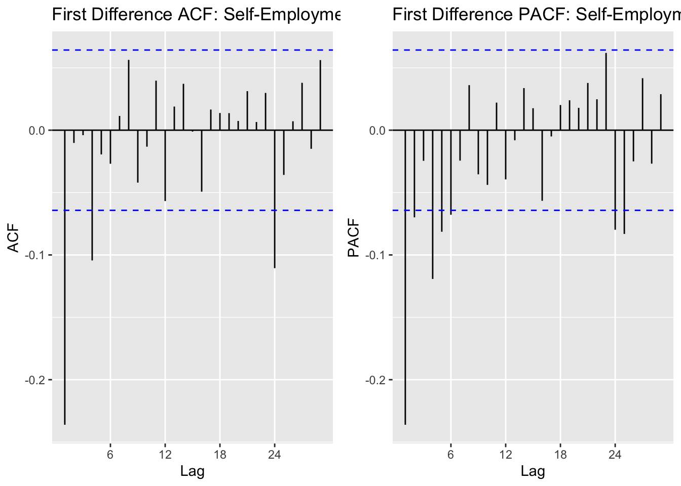
The ACF shows strong autocorrelation at seasonal lags (12, 24), suggesting seasonal differencing may be needed. The PACF shows significant spikes at early lags, indicating AR terms. Given the monthly data with clear seasonal patterns, we’ll explore SARIMA models.
Show Code
# Run model comparisonoutput_se =SARIMA.c(p1 =0, p2 =3, q1 =0, q2 =3, P1 =0, P2 =2, Q1 =0, Q2 =2, data = self_emp.ts)# Identify best modelsminaic_se = output_se[which.min(output_se$AIC), ]minbic_se = output_se[which.min(output_se$BIC), ]print("Best Model Based on AIC:")
[1] "Best Model Based on AIC:"
Show Code
print(minaic_se)
    p d q P D Q      AIC      BIC     AICc
131 3 1 2 2 1 1 11536.25 11579.66 11536.45
Show Code
print("Best Model Based on BIC:")
[1] "Best Model Based on BIC:"
Show Code
print(minbic_se)
   p d q P D Q      AIC      BIC     AICc
17 0 1 1 2 1 1 11545.31 11569.43 11545.38
Show Code
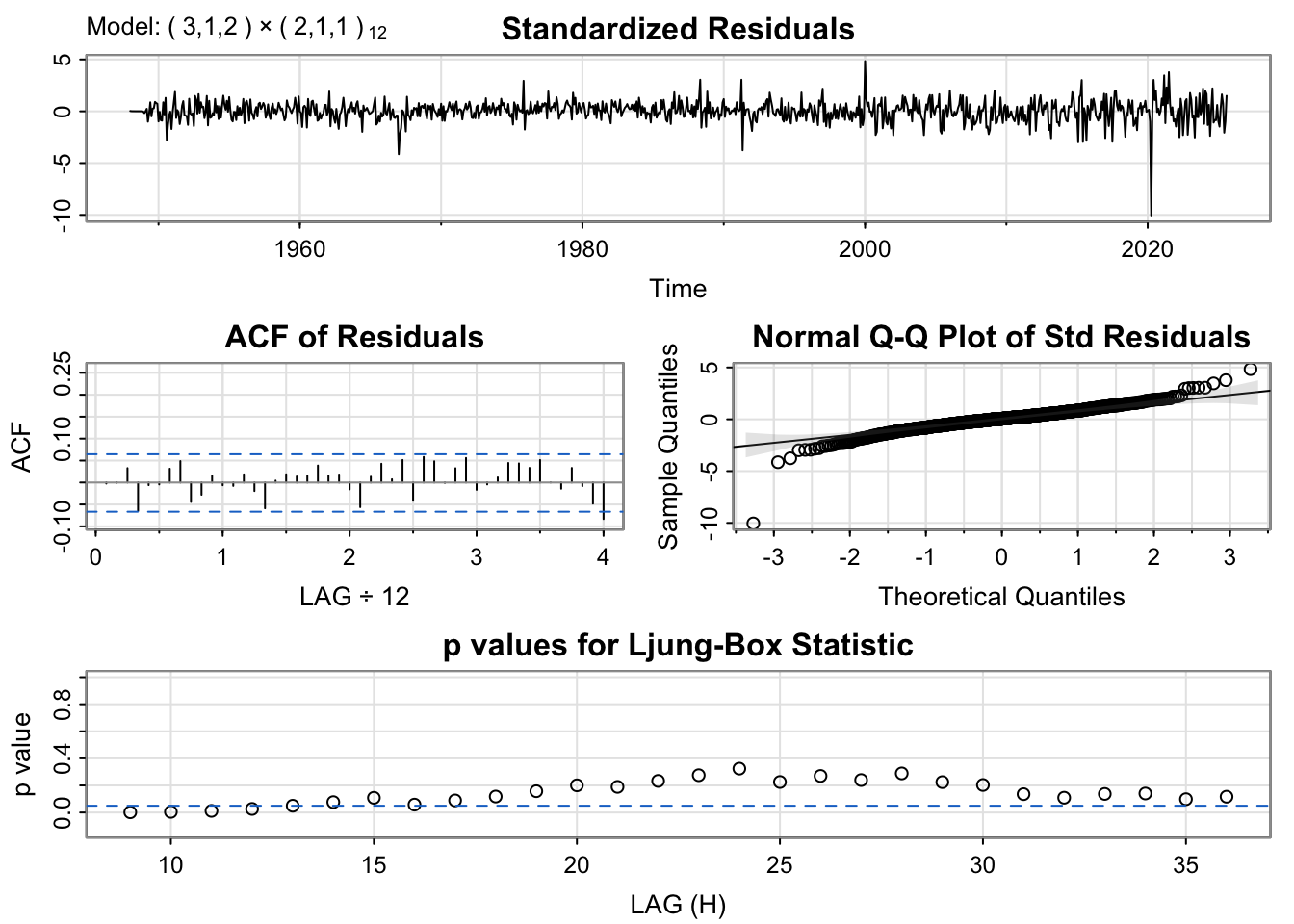
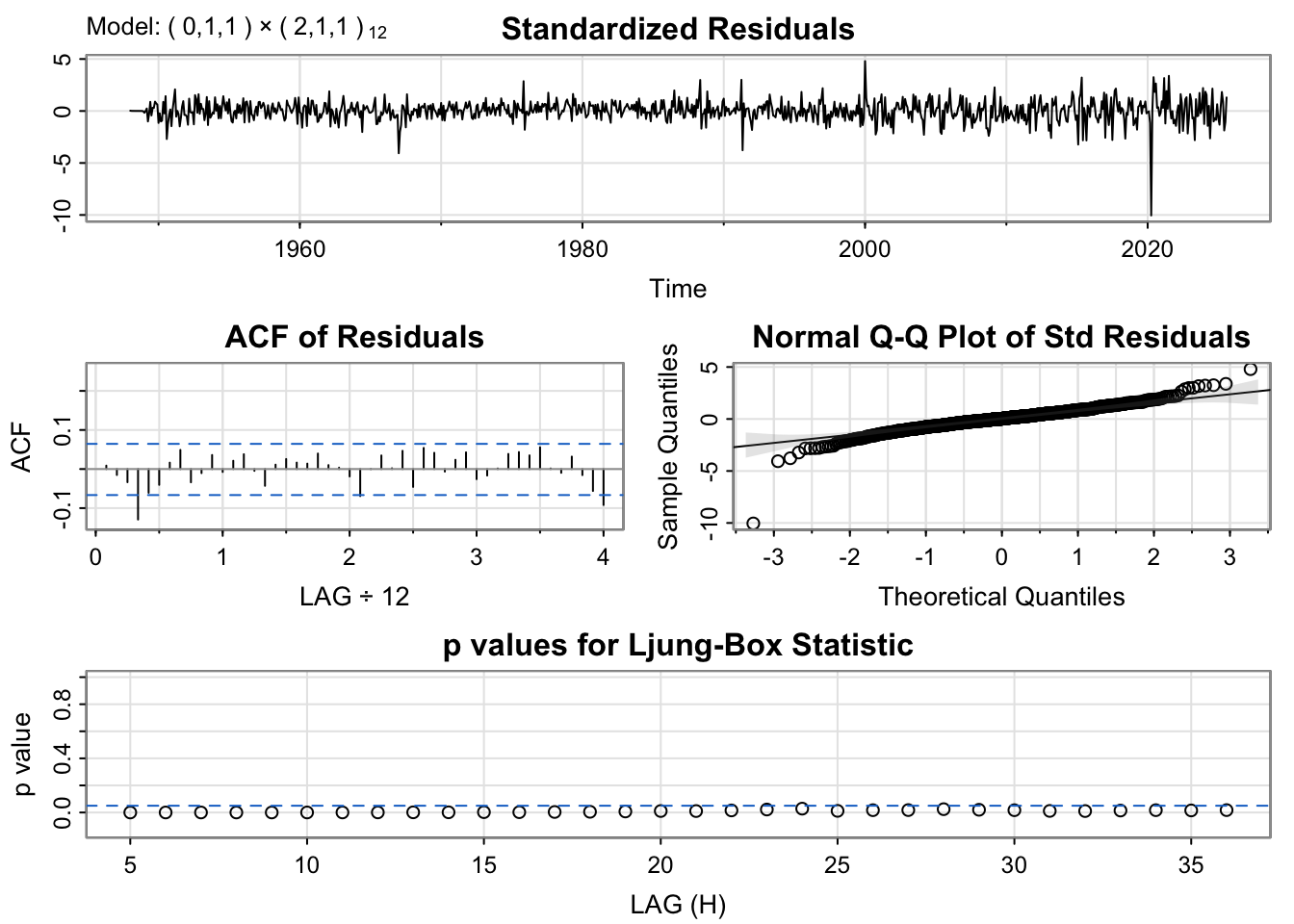
# Run diagnostics for top candidatesmodel_1_se_output <-capture.output(sarima(self_emp.ts, minaic_se$p, minaic_se$d, minaic_se$q, minaic_se$P, minaic_se$D, minaic_se$Q, 12))
The diagnostic plots show well-behaved residuals for both models. We’ll select the BIC model for parsimony and better generalization to future data.
Show Code
# Fit the selected modelfit_se <-Arima(self_emp.ts, order =c(minbic_se$p, minbic_se$d, minbic_se$q),seasonal =list(order=c(minbic_se$P, minbic_se$D, minbic_se$Q), period=12))summary(fit_se)
Series: self_emp.ts
ARIMA(0,1,1)(2,1,1)[12]

Coefficients:
          ma1     sar1     sar2     sma1
      -0.2685  -0.0476  -0.1285  -1.0000
s.e.   0.0340   0.0332   0.0336   0.0499

sigma^2 = 15631:  log likelihood = -5767.66
AIC=11545.31   AICc=11545.38   BIC=11569.43

Training set error measures:
                   ME   RMSE      MAE        MPE     MAPE      MASE        ACF1
Training set 2.493403 123.88 87.98592 0.02793437 1.169764 0.4097278 0.008738898
Show Code
# Generate 36-month forecastfc_se_arima <-forecast(fit_se, h =36)# Benchmark modelsfc_se_naive <-naive(self_emp.ts, h =36)fc_se_snaive <-snaive(self_emp.ts, h =36)fc_se_ets <-forecast(ets(self_emp.ts), h =36)fc_se_drift <-rwf(self_emp.ts, h =36, drift =TRUE)# Plot all forecastsautoplot(self_emp.ts) +autolayer(fc_se_arima, series =paste0("ARIMA(", minbic_se$p, ",", minbic_se$d, ",", minbic_se$q,")(", minbic_se$P, ",", minbic_se$D, ",", minbic_se$Q, ")[12]"), PI =FALSE) +autolayer(fc_se_ets, series ="ETS", PI =FALSE, alpha=0.7) +autolayer(fc_se_drift, series ="Drift", PI =FALSE, alpha=0.7) +autolayer(fc_se_naive, series ="Naive", PI =FALSE, alpha=0.7) +autolayer(fc_se_snaive, series ="Seasonal Naive", PI =FALSE, alpha=0.7) +labs(title ="Self-Employment: \n36-Month Forecast Comparison",y ="Self-Employed Persons (Thousands)",x ="Year" ) +guides(colour =guide_legend(title ="Forecast Method"))
The self-employment forecast reveals critical insights for our entrepreneurship narrative. The ARIMA model projects relatively flat growth over the next 36 months, continuing the pattern of stagnation observed since the 2008-2010 period. This is particularly significant given that this stagnation coincides precisely with the exponential growth in student loan debt.
Prior to 2008, self-employment showed steady growth, representing a viable wealth-building pathway for Americans. However, the post-2008 flattening suggests that rising educational debt burdens may be blocking young people from taking the entrepreneurial leap - they cannot afford the risk when carrying substantial debt obligations. This finding will be further explored in our multivariate models and interrupted time series analysis, where we can test whether student debt Granger-causes declines in entrepreneurship.
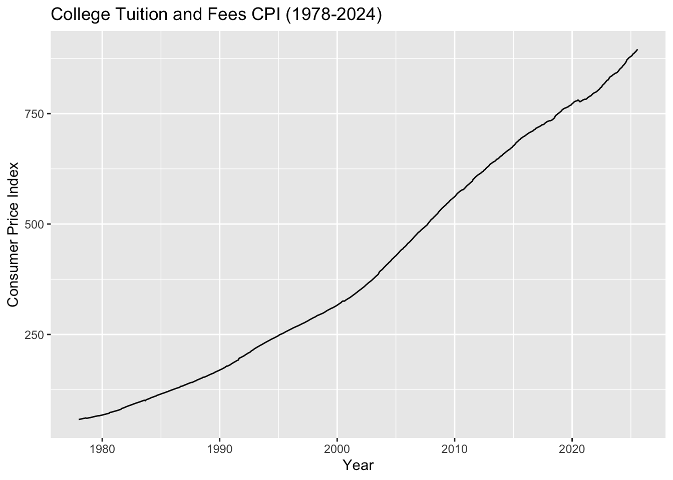
The College Tuition and Fees Consumer Price Index (1978-2024, 552 monthly observations) explains the root cause of the student debt crisis. This dataset shows tuition costs increased approximately 1500% while median household income only grew 25% over a similar period.
Show Code
# Load college tuition CPI datacollege_tuition <-read.csv('data/raw/CUSR0000SEEB.csv')# Create time series objecttuition.ts <-ts(college_tuition$CUSR0000SEEB, start =c(1978, 1), frequency =12)# Plot the full seriesautoplot(tuition.ts) +labs(title ="College Tuition and Fees CPI (1978-2024)",y ="Consumer Price Index",x ="Year" )
The tuition CPI shows a relentless upward trend with no sign of leveling off. This exponential growth far outpaces inflation and income growth, making higher education increasingly unaffordable without taking on debt. The trend appears highly non-stationary and will likely require differencing.
The ACF shows some remaining autocorrelation after first differencing, with seasonal patterns visible. The PACF shows significant spikes at early lags. We’ll test SARIMA models to capture both the trend and seasonal components.
Show Code
# Run model comparisonoutput_tuit =SARIMA.c(p1 =0, p2 =3, q1 =0, q2 =3, P1 =0, P2 =2, Q1 =0, Q2 =2, data = tuition.ts)# Identify best modelsminaic_tuit = output_tuit[which.min(output_tuit$AIC), ]minbic_tuit = output_tuit[which.min(output_tuit$BIC), ]print("Best Model Based on AIC:")
[1] "Best Model Based on AIC:"
Show Code
print(minaic_tuit)
   p d q P D Q      AIC     BIC    AICc
54 1 1 1 2 1 2 1072.257 1102.54 1072.46
Show Code
print("Best Model Based on BIC:")
[1] "Best Model Based on BIC:"
Show Code
print(minbic_tuit)
   p d q P D Q      AIC     BIC    AICc
54 1 1 1 2 1 2 1072.257 1102.54 1072.46
Show Code
# Run diagnostics for top candidatesmodel_1_tuit_output <-capture.output(sarima(tuition.ts, minaic_tuit$p, minaic_tuit$d, minaic_tuit$q, minaic_tuit$P, minaic_tuit$D, minaic_tuit$Q, 12))
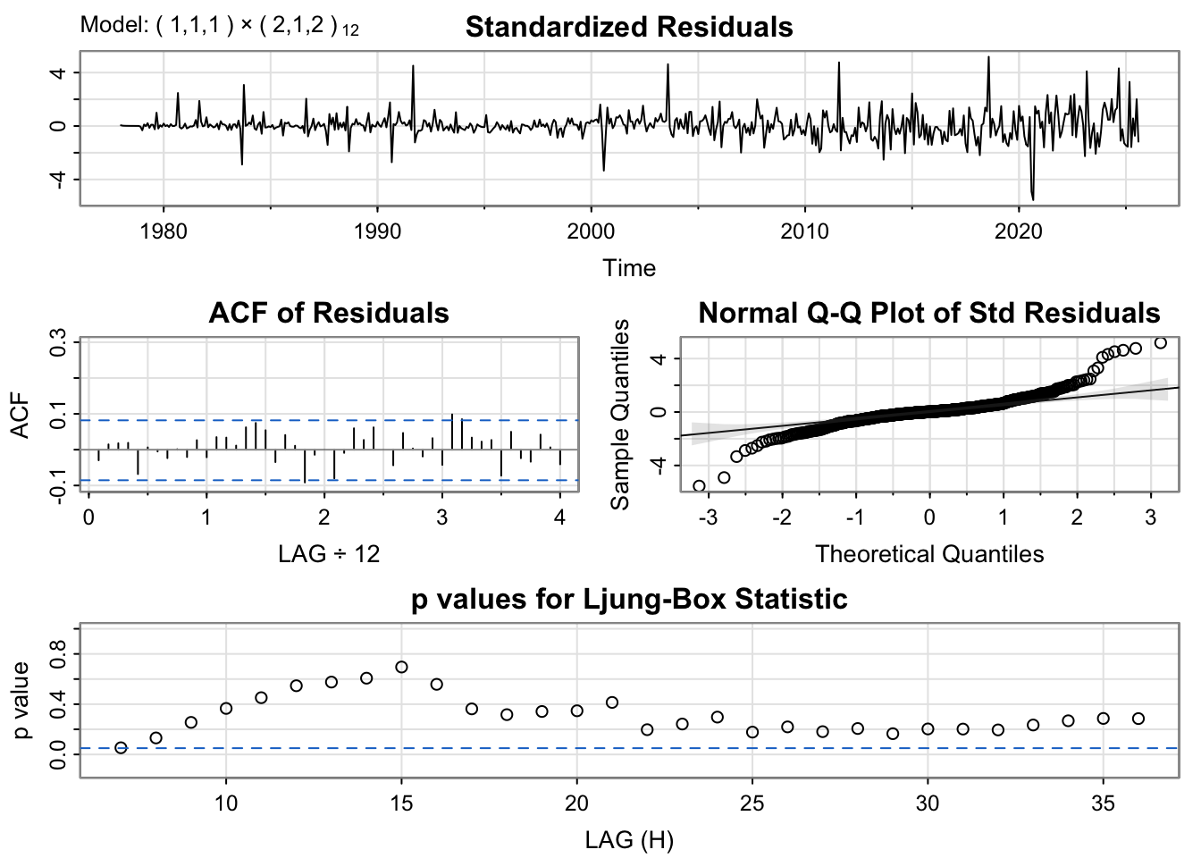
The diagnostic plots confirm both models have well-behaved residuals. We’ll use the BIC model for better generalization.
Show Code
# Fit the selected modelfit_tuit <-Arima(tuition.ts, order =c(minbic_tuit$p, minbic_tuit$d, minbic_tuit$q),seasonal =list(order=c(minbic_tuit$P, minbic_tuit$D, minbic_tuit$Q), period=12))summary(fit_tuit)
Series: tuition.ts
ARIMA(1,1,1)(2,1,2)[12]

Coefficients:
         ar1      ma1    sar1     sar2     sma1    sma2
      0.9974  -0.8607  0.4595  -0.1407  -1.6264  0.6477
s.e.  0.0037   0.0214  0.1011   0.0523   0.0952  0.0947

sigma^2 = 0.3653:  log likelihood = -529.13
AIC=1072.26   AICc=1072.46   BIC=1102.54

Training set error measures:
                     ME      RMSE       MAE        MPE      MAPE       MASE
Training set 0.02594605 0.5943104 0.3755686 0.01796685 0.1105055 0.02128406
                    ACF1
Training set -0.02955446
Show Code
# Generate 36-month forecastfc_tuit_arima <-forecast(fit_tuit, h =36)# Benchmark modelsfc_tuit_naive <-naive(tuition.ts, h =36)fc_tuit_snaive <-snaive(tuition.ts, h =36)fc_tuit_ets <-forecast(ets(tuition.ts), h =36)fc_tuit_drift <-rwf(tuition.ts, h =36, drift =TRUE)# Plot all forecastsautoplot(tuition.ts) +autolayer(fc_tuit_arima, series =paste0("ARIMA(", minbic_tuit$p, ",", minbic_tuit$d, ",", minbic_tuit$q,")(", minbic_tuit$P, ",", minbic_tuit$D, ",", minbic_tuit$Q, ")[12]"), PI =FALSE) +autolayer(fc_tuit_ets, series ="ETS", PI =FALSE) +autolayer(fc_tuit_drift, series ="Drift", PI =FALSE) +autolayer(fc_tuit_naive, series ="Naive", PI =FALSE) +autolayer(fc_tuit_snaive, series ="Seasonal Naive", PI =FALSE) +labs(title ="College Tuition CPI: \n36-Month Forecast Comparison",y ="Consumer Price Index",x ="Year" ) +guides(colour =guide_legend(title ="Forecast Method"))
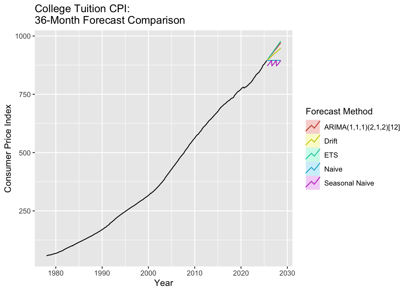
The tuition CPI forecast shows continued growth over the next 36 months, though the rate of increase appears to be moderating slightly compared to historical trends. This continued upward trajectory means that even if student loan forgiveness programs were implemented, future students would still face the same affordability crisis unless tuition growth is addressed at its source.
The forecast underscores why student debt has become unavoidable for most Americans seeking higher education - when costs increase 15x over four decades while incomes remain relatively flat, debt becomes the only viable option for accessing educational opportunities.
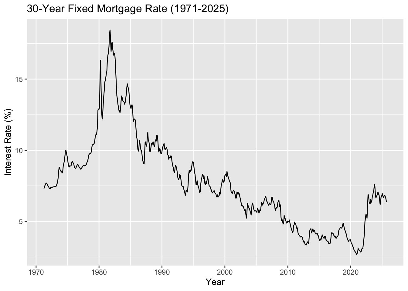
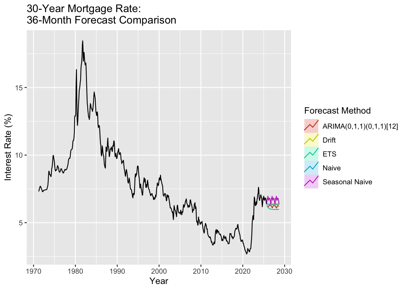
The 30-year fixed mortgage rate (1971-2025, aggregated from weekly to monthly) shows the cost of borrowing for homeownership. Recent rate increases (3% to 7% in 2022-2024) create a triple threat for debt-burdened millennials: high student debt, high housing prices, and now high borrowing costs.
Show Code
# Load mortgage rate data (weekly)mortgage_rates <-read.csv('data/raw/MORTGAGE30US.csv')mortgage_rates$observation_date <-as.Date(mortgage_rates$observation_date)# Aggregate to monthly (take mean of weekly rates)mortgage_monthly <- mortgage_rates %>%mutate(year_month =format(observation_date, "%Y-%m")) %>%group_by(year_month) %>%summarise(avg_rate =mean(MORTGAGE30US, na.rm =TRUE), .groups ='drop') %>%mutate(date =as.Date(paste0(year_month, "-01"))) %>%arrange(date)# Create time series object (starts April 1971)mortgage.ts <-ts(mortgage_monthly$avg_rate, start =c(1971, 4), frequency =12)# Plot the full seriesautoplot(mortgage.ts) +labs(title ="30-Year Fixed Mortgage Rate (1971-2025)",y ="Interest Rate (%)",x ="Year" )
Mortgage rates show dramatic historical volatility, peaking above 18% in the early 1980s, declining to historic lows around 3% in 2020-2021, then doubling to 7% by 2023-2024. This recent spike makes homeownership particularly challenging for young adults already carrying student debt burdens.
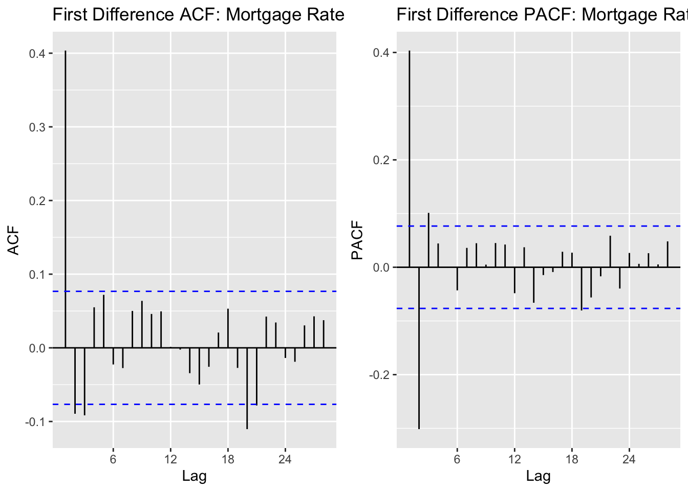
The ACF shows strong autocorrelation at lag 1, then cuts off, suggesting MA(1) behavior. The PACF shows significant spikes at early lags, suggesting AR terms. Mortgage rates are known to exhibit strong mean reversion, which should be captured by the AR component.
Show Code
# Run model comparisonoutput_mort =SARIMA.c(p1 =0, p2 =3, q1 =0, q2 =3, P1 =0, P2 =1, Q1 =0, Q2 =1, data = mortgage.ts)# Identify best modelsminaic_mort = output_mort[which.min(output_mort$AIC), ]minbic_mort = output_mort[which.min(output_mort$BIC), ]print("Best Model Based on AIC:")
[1] "Best Model Based on AIC:"
Show Code
print(minaic_mort)
   p d q P D Q      AIC      BIC    AICc
50 3 1 0 0 1 1 35.68521 58.00036 35.7797
Show Code
print("Best Model Based on BIC:")
[1] "Best Model Based on BIC:"
Show Code
print(minbic_mort)
  p d q P D Q      AIC     BIC     AICc
6 0 1 1 0 1 1 43.30751 56.6966 43.34519
Show Code
# Run diagnostics for top candidatesmodel_1_mort_output <-capture.output(sarima(mortgage.ts, minaic_mort$p, minaic_mort$d, minaic_mort$q, minaic_mort$P, minaic_mort$D, minaic_mort$Q, 12))
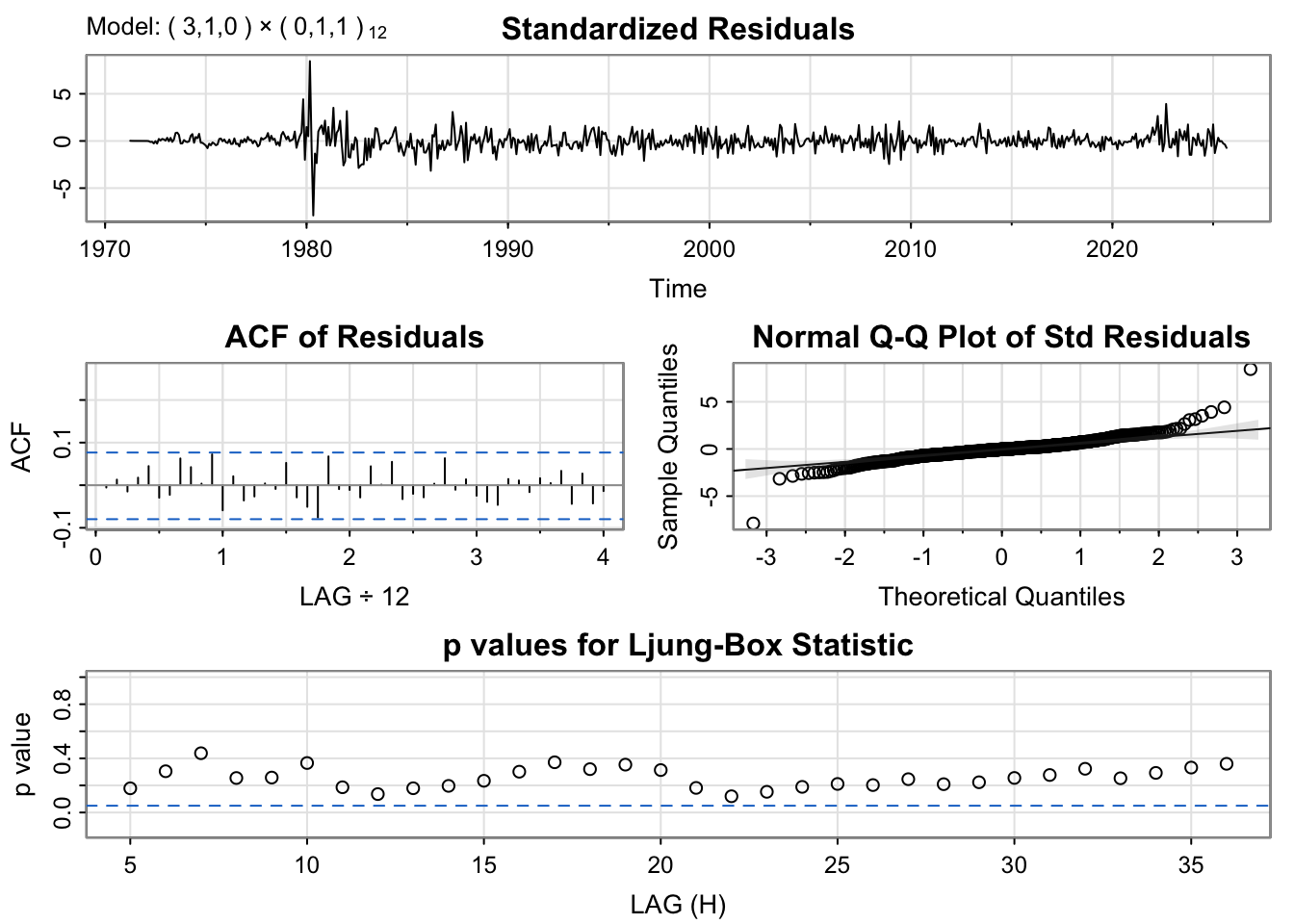
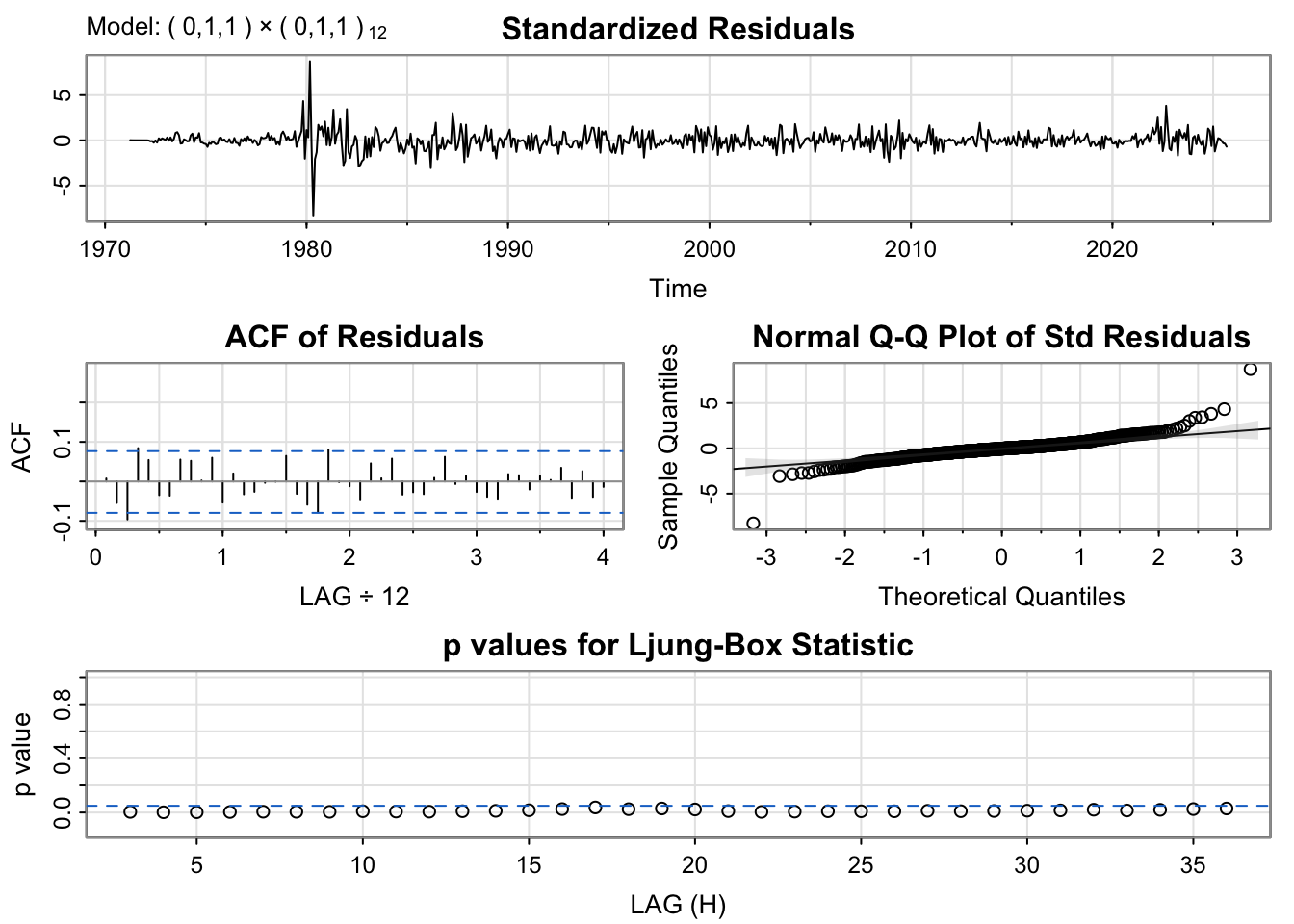
Diagnostic plots indicate well-behaved residuals. We’ll select the BIC model for parsimony.
Show Code
# Fit the selected modelfit_mort <-Arima(mortgage.ts, order =c(minbic_mort$p, minbic_mort$d, minbic_mort$q),seasonal =list(order=c(minbic_mort$P, minbic_mort$D, minbic_mort$Q), period=12))summary(fit_mort)
Series: mortgage.ts
ARIMA(0,1,1)(0,1,1)[12]

Coefficients:
         ma1     sma1
      0.5376  -1.0000
s.e.  0.0314   0.0334

sigma^2 = 0.05774:  log likelihood = -18.65
AIC=43.31   AICc=43.35   BIC=56.7

Training set error measures:
                      ME      RMSE       MAE         MPE     MAPE      MASE
Training set -0.00712295 0.2375107 0.1553439 -0.06839809 2.135183 0.1812716
                    ACF1
Training set 0.007485004
Show Code
# Generate 36-month forecastfc_mort_arima <-forecast(fit_mort, h =36)# Benchmark modelsfc_mort_naive <-naive(mortgage.ts, h =36)fc_mort_snaive <-snaive(mortgage.ts, h =36)fc_mort_ets <-forecast(ets(mortgage.ts), h =36)fc_mort_drift <-rwf(mortgage.ts, h =36, drift =TRUE)# Plot all forecastsautoplot(mortgage.ts) +autolayer(fc_mort_arima, series =paste0("ARIMA(", minbic_mort$p, ",", minbic_mort$d, ",", minbic_mort$q,")(", minbic_mort$P, ",", minbic_mort$D, ",", minbic_mort$Q, ")[12]"), PI =FALSE) +autolayer(fc_mort_ets, series ="ETS", PI =FALSE) +autolayer(fc_mort_drift, series ="Drift", PI =FALSE) +autolayer(fc_mort_naive, series ="Naive", PI =FALSE) +autolayer(fc_mort_snaive, series ="Seasonal Naive", PI =FALSE) +labs(title ="30-Year Mortgage Rate: \n36-Month Forecast Comparison",y ="Interest Rate (%)",x ="Year" ) +guides(colour =guide_legend(title ="Forecast Method"))
The mortgage rate forecast has critical implications for our housing affordability narrative. If rates remain elevated (as the ARIMA model suggests they will over the next 36 months), the combination of high student debt + high housing prices + high mortgage rates creates an unprecedented affordability crisis.
For context: a $400,000 home at 3% interest has a monthly payment of $1,686. The same home at 7% costs $2,661 per month - a 58% increase. For millennials already paying $300-500/month in student loans, this rate difference can be the deciding factor between homeownership and continued renting, perpetuating the wealth gap between debt-burdened and debt-free individuals.
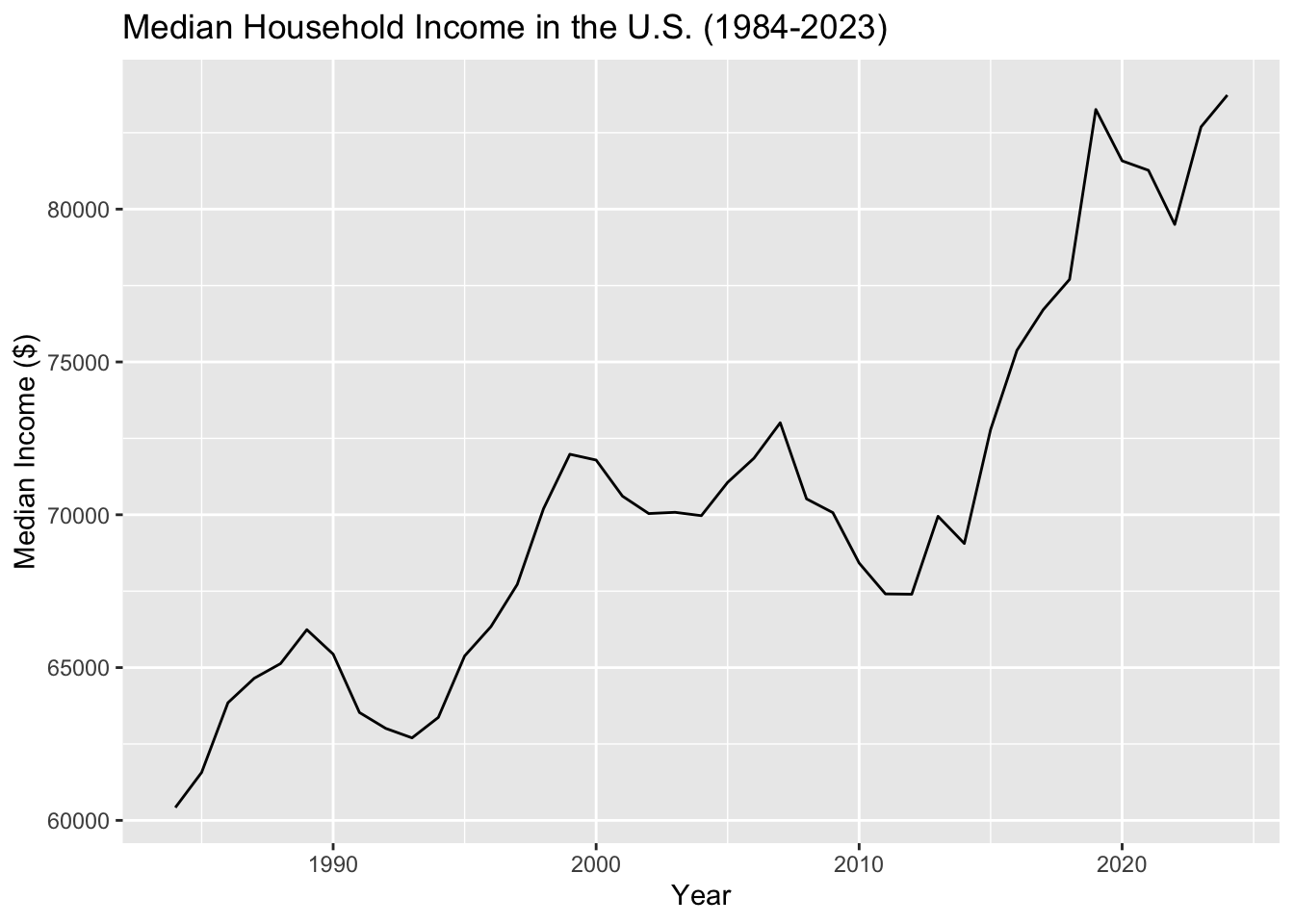
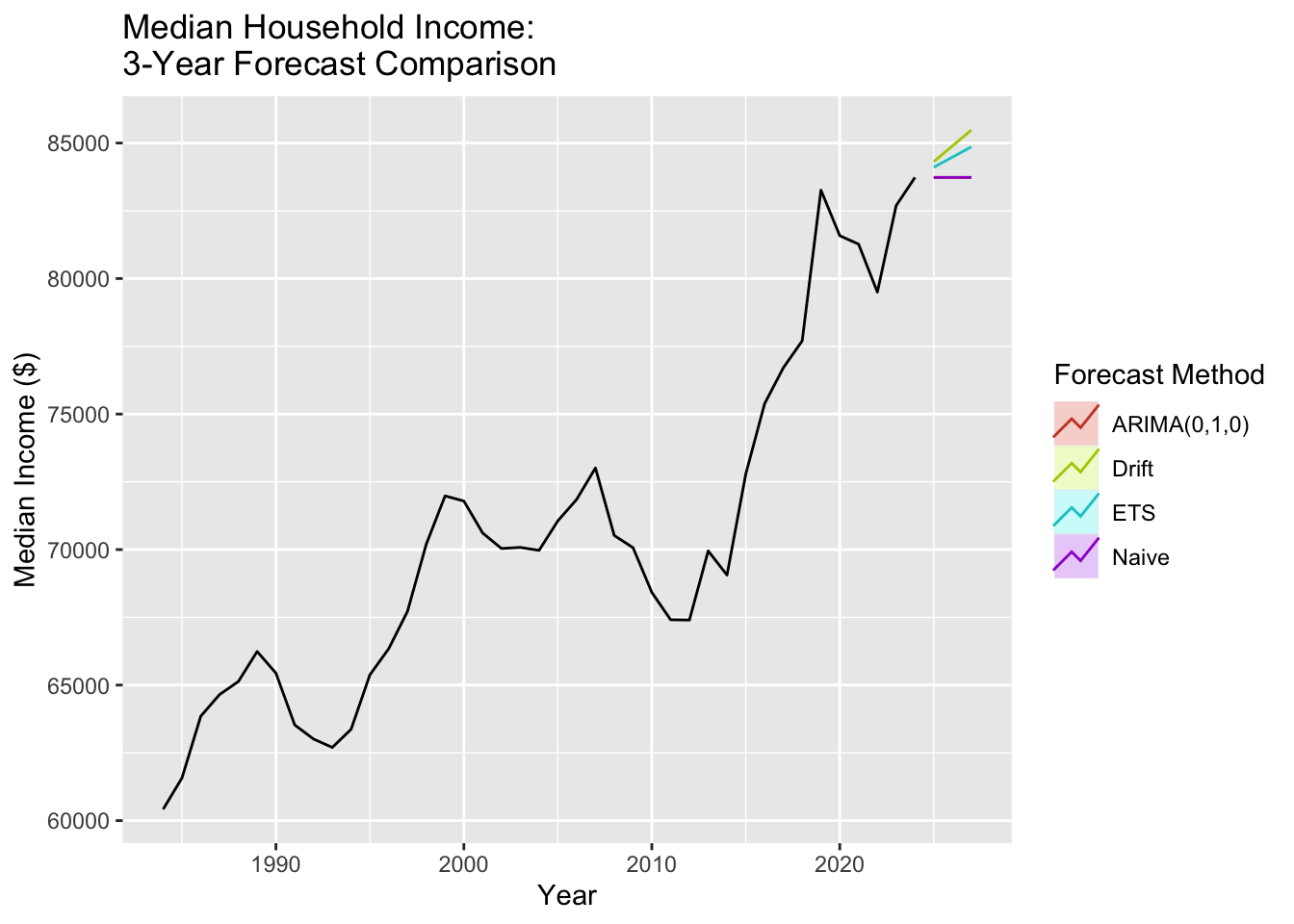
Median household income (1984-2023, annual data) is the denominator in every affordability calculation. While tuition increased 1500% and housing increased 300%, median income only grew approximately 25% over similar periods. This mismatch explains why debt has become unavoidable.
Show Code
# Load median household income datamedian_income <-read.csv('data/raw/MEHOINUSA672N.csv')# Create time series object (annual data, no seasonal component)income.ts <-ts(median_income$MEHOINUSA672N, start =1984, frequency =1)# Plot the full seriesautoplot(income.ts) +labs(title ="Median Household Income in the U.S. (1984-2023)",y ="Median Income ($)",x ="Year" )
The income data shows modest growth with a dip during the 2008 financial crisis and subsequent recovery. However, the absolute growth in dollars has not kept pace with cost increases in education and housing, creating an affordability squeeze.
Show Code
# ACF and PACF for first-differenced datap1 <-ggAcf(diff(income.ts, differences =1)) +labs(title ="First Difference ACF: Median Income")p2 <-ggPacf(diff(income.ts, differences =1)) +labs(title ="First Difference PACF: Median Income")grid.arrange(p1, p2, nrow=1, ncol=2)
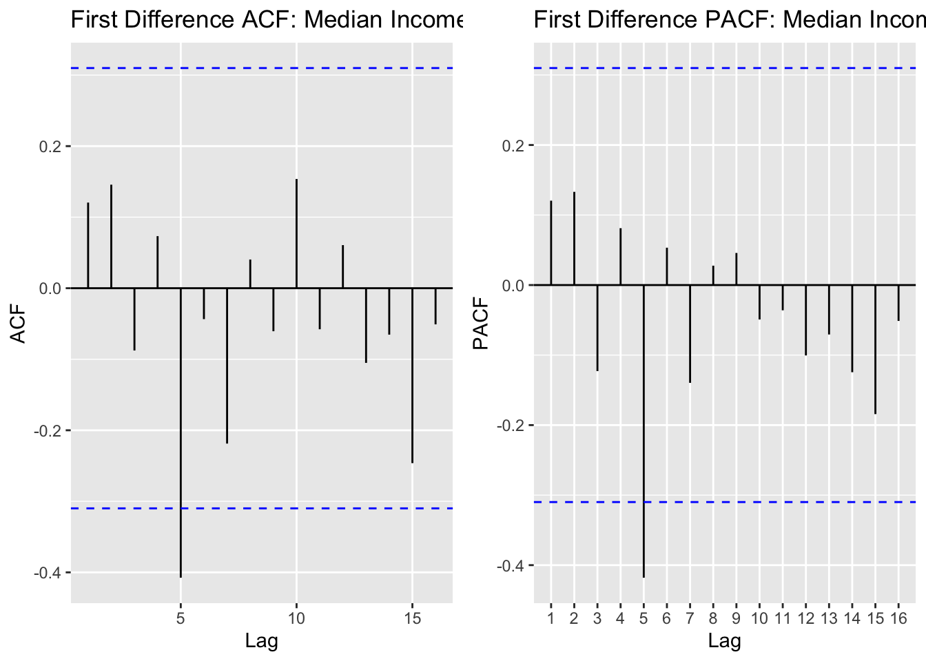
With only 42 annual observations, we see limited autocorrelation structure. The ACF shows a few significant lags early on, and the PACF shows a spike at lag 1. We’ll test simple ARIMA models without seasonal components.
Show Code
# Create a simpler comparison function for annual data (no seasonal components)ARIMA_annual <-function(p_max, q_max, data) { d <-1 results <-data.frame()for (p in0:p_max) {for (q in0:q_max) {if (p + d + q <=4) { # Keep models simple for limited data fit <-tryCatch(Arima(data, order =c(p, d, q)),error =function(e) NULL )if (!is.null(fit)) { results <-rbind(results, data.frame(p = p, d = d, q = q,AIC = fit$aic, BIC = fit$bic, AICc = fit$aicc )) } } } }return(results)}# Run model comparison (smaller ranges for annual data)output_inc <-ARIMA_annual(p_max =3, q_max =3, data = income.ts)# Identify best modelsminaic_inc = output_inc[which.min(output_inc$AIC), ]minbic_inc = output_inc[which.min(output_inc$BIC), ]print("Best Model Based on AIC:")
[1] "Best Model Based on AIC:"
Show Code
print(minaic_inc)
  p d q      AIC      BIC     AICc
9 2 1 1 710.9203 717.6758 712.0631
Show Code
print("Best Model Based on BIC:")
[1] "Best Model Based on BIC:"
Show Code
print(minbic_inc)
  p d q      AIC      BIC     AICc
1 0 1 0 713.3494 715.0383 713.4547
Show Code
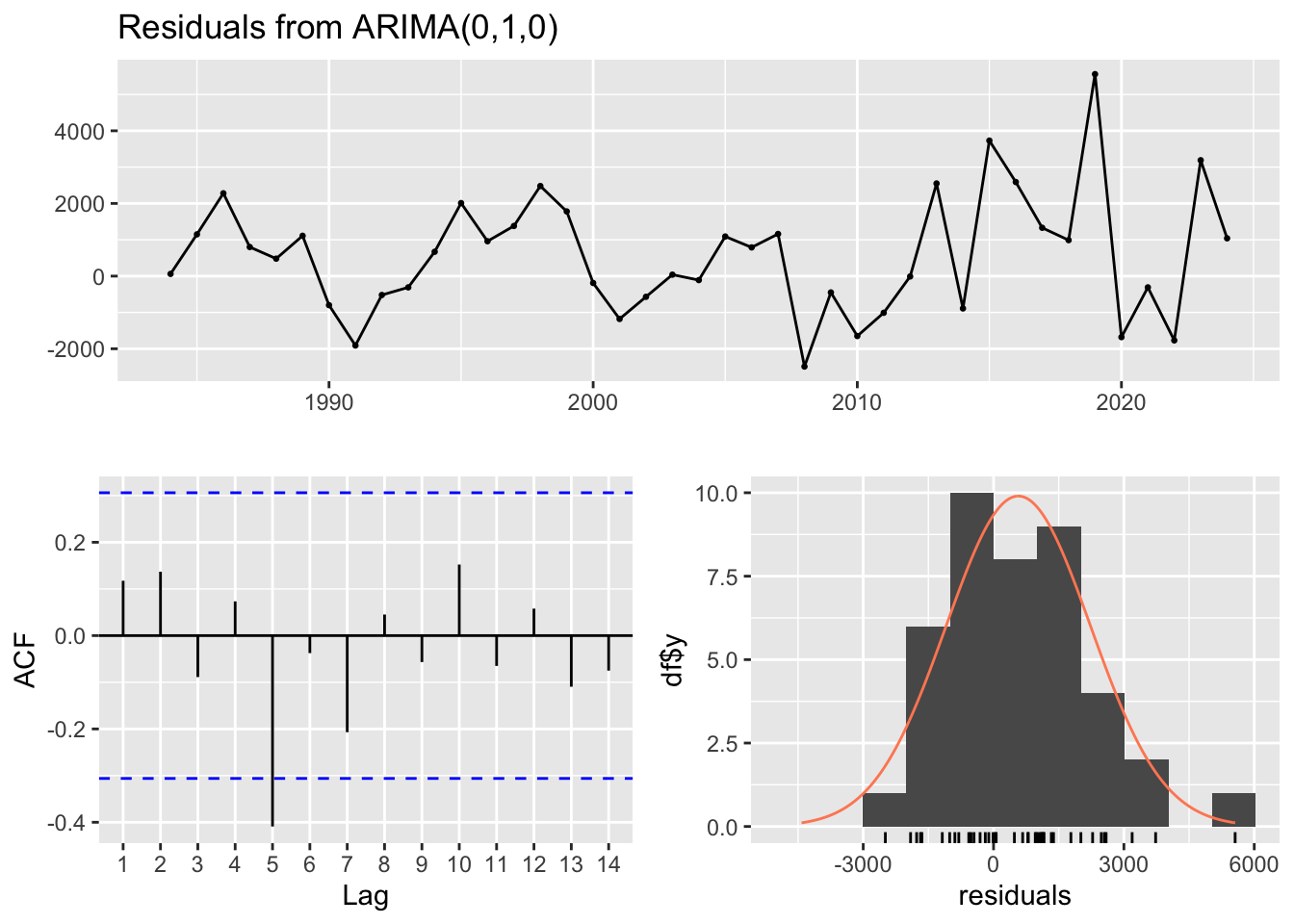
# Fit models for diagnostics (annual data is limited, so use simpler diagnostics)fit_inc_aic <-Arima(income.ts, order =c(minaic_inc$p, minaic_inc$d, minaic_inc$q))fit_inc_bic <-Arima(income.ts, order =c(minbic_inc$p, minbic_inc$d, minbic_inc$q))# Check residuals for BIC modelcheckresiduals(fit_inc_bic)
    Ljung-Box test

data:  Residuals from ARIMA(0,1,0)
Q* = 12.672, df = 8, p-value = 0.1236

Model df: 0.   Total lags used: 8
The diagnostic plots show the residuals are reasonably well-behaved given the limited annual data. We’ll use the BIC model for its parsimony.
Show Code
# Fit the selected modelfit_inc <-Arima(income.ts, order =c(minbic_inc$p, minbic_inc$d, minbic_inc$q))summary(fit_inc)
Series: income.ts
ARIMA(0,1,0)

sigma^2 = 3096824:  log likelihood = -355.67
AIC=713.35   AICc=713.45   BIC=715.04

Training set error measures:
                   ME     RMSE      MAE       MPE     MAPE      MASE      ACF1
Training set 570.0102 1738.186 1343.181 0.7700606 1.868072 0.9766813 0.1175003
Show Code
# Generate 3-year forecast (annual data, so h=3)fc_inc_arima <-forecast(fit_inc, h =3)# Benchmark modelsfc_inc_naive <-naive(income.ts, h =3)fc_inc_ets <-forecast(ets(income.ts), h =3)fc_inc_drift <-rwf(income.ts, h =3, drift =TRUE)# Plot all forecastsautoplot(income.ts) +autolayer(fc_inc_arima, series =paste0("ARIMA(", minbic_inc$p, ",", minbic_inc$d, ",", minbic_inc$q, ")"), PI =FALSE) +autolayer(fc_inc_ets, series ="ETS", PI =FALSE) +autolayer(fc_inc_drift, series ="Drift", PI =FALSE) +autolayer(fc_inc_naive, series ="Naive", PI =FALSE) +labs(title ="Median Household Income: \n3-Year Forecast Comparison",y ="Median Income ($)",x ="Year" ) +guides(colour =guide_legend(title ="Forecast Method"))
The median income forecast shows continued modest growth over the next 3 years. However, this growth rate remains far below the growth rates of tuition and housing costs. If income grows 2-3% annually while tuition grows 5-6% annually, the affordability gap continues to widen each year.
This dataset serves as the crucial context for understanding why student debt has exploded: not because students are making poor decisions, but because the economic fundamentals have shifted dramatically against them. The “pull yourself up by your bootstraps” narrative breaks down when bootstraps cost 1500% more while your paycheck only grows 25%.
Source Code
---title: "Univariate TS Model (ARIMA, SARIMA)"execute: warning: false message: false error: false---This section applies univariate time series models to the key variables, focusing on ARIMA (AutoRegressive Integrated Moving Average) and SARIMA (Seasonal ARIMA) frameworks. These models capture autocorrelation, trend, and seasonality within individual series without considering relationships between variables. By systematically identifying model orders through ACF/PACF analysis and information criteria, I establish baseline forecasts and understand the inherent dynamics of student loan debt, homeownership rates, and related economic indicators.```{r include=FALSE}#| include: false#| echo: false#| output: falselibrary(rvest)library(dplyr)library(tidyr)library(stringr)library(purrr)library(glue)library(readr)library(tidyverse)library(ggplot2)library(forecast)library(astsa) library(xts)library(tseries)library(fpp2)library(fma)library(lubridate)library(TSstudio)library(quantmod)library(tidyquant)library(plotly)library(ggplot2)library(readxl)library(gridExtra)``````{r include=FALSE}bronxville_b_long <- read.csv('data/processed/bronxville_b_long.csv')bronxville_t_long <- read.csv('data/processed/bronxville_t_long.csv')mv_b_long <- read.csv('data/processed/mount_vernon_b_long.csv')mv_t_long <- read.csv('data/processed/mount_vernon_t_long.csv')hpi_us <- read.csv('data/processed/hpi_us.csv')slq <- read.csv('data/processed/student_loans_q.csv')``````{r include=FALSE} SARIMA.c <- function(p1, p2, q1, q2, P1, P2, Q1, Q2, data) { # differencing & seasonal period d <- 1; D <- 1; s <- 12 # preallocate max_rows <- (p2 - p1 + 1) * (q2 - q1 + 1) * (P2 - P1 + 1) * (Q2 - Q1 + 1) results_matrix <- matrix(NA_real_, nrow = max_rows, ncol = 9) i <- 1 for (p in p1:p2) { for (q in q1:q2) { for (P in P1:P2) { for (Q in Q1:Q2) { # parameter constraint if (p + d + q + P + D + Q <= 10) { fit <- tryCatch( Arima( data, order = c(p, d, q), seasonal = list(order = c(P, D, Q), period = s) ), error = function(e) NULL ) if (!is.null(fit)) { results_matrix[i, ] <- c(p, d, q, P, D, Q, fit$aic, fit$bic, fit$aicc) i <- i + 1 } } } } } } # keep only filled rows if (i == 1) { stop("No models were successfully fitted. Check seasonal period/frequency and parameter ranges.") } results_df <- as.data.frame(results_matrix[1:(i - 1), , drop = FALSE]) names(results_df) <- c("p","d","q","P","D","Q","AIC","BIC","AICc") return(results_df) }``````{r include+FALSE}hpi.ts <- ts(hpi_us$index_nsa, start=c(1991,01), frequency = 12)mv_b.ts <- ts(mv_b_long$hvi, start=c(2000,01), frequency = 12)mv_t.ts <- ts(mv_t_long$hvi, start=c(2000,01), frequency = 12)bronxville_b.ts <- ts(bronxville_b_long$hvi, start=c(2000,01), frequency = 12)bronxville_b.ts <- window(bronxville_b.ts, start=c(2016,02), end=c(2025,08), frequency = 12)bronxville_t.ts <- ts(bronxville_t_long$hvi, start=c(2000,01), frequency = 12)bronxville_t.ts <- window(bronxville_t.ts, start=c(2016,02), end=c(2025,08), frequency = 12)slq.ts <- ts(slq$SLOASM, start=c(2006,03), frequency = 12)```## U.S. Housing Price Index::: {.panel-tabset}### Overview & Time Series```{r}#| echo: false#| warning: false# Plot the U.S. Housing Price Index time seriesautoplot(hpi.ts) +labs(title ="U.S. Housing Price Index (1991-2024)",y ="Home Price Index (NSA)",x ="Year" ) +theme_minimal()```The U.S. Housing Price Index shows the dramatic boom-bust cycle from the 2008 housing crisis, followed by a strong recovery and the COVID-era surge to new peaks in 2021-2022, before recent corrections as mortgage rates increased.### ACF/PACF Analysis```{r}#| echo: false#| warning: false#housing price index## seasonal differenceseas_diff_hpi <-diff(diff(hpi.ts, differences =1), lag =12)p1 <-ggAcf(diff(hpi.ts), 50) +labs(title ='First Order Differencing ACF \nfor Housing Price Index')p2 <-ggAcf(seas_diff_hpi, 50) +labs(title ="Seasonal Difference ACF Plot \nfor Housing Price Index")p3 <-ggPacf(diff(hpi.ts), 50) +labs(title ='First Order Differencing PACF \nfor Housing Price Index')p4 <-ggPacf(seas_diff_hpi, 50) +labs(title ="Seasonal Difference PACF Plot \nfor Housing Price Index")grid.arrange(p1, p3, nrow=2)grid.arrange(p2, p4)```After seasonal differencing, the lag for both ACF and PACF appear to display removed autocorrelation and shock. This shows that first differencing managed to remove the trend and seasonality, leaving a fully stationary series and virtually no autocorrelation. For modeling, I will test the following values for p,d,q:p = 1,2d = 1q = 1,2,3P = 1,2D = 1Q = 1,2,3### Model Comparison```{r}#| echo: false#| warning: false# p = 1:3, P = 1,2, q = 1:4 , Q = 1:5: : d = 1 , D = 1###### Run SARIMA Model Comparison ###### output =SARIMA.c(p1 =1, p2 =3, q1 =1, q2 =4, P1 =1, P2 =2, Q1 =1, Q2 =5, data = hpi.ts)###### Identify Models with Minimum AIC and BIC ###### minaic = output[which.min(output$AIC), ] minbic = output[which.min(output$BIC), ]###### Display Best Models Based on AIC and BIC ######print("Best Model Based on AIC:")print(minaic)print("Best Model Based on BIC:")print(minbic)``````{r}extract_model_output <-function(model_output, model_name) { start_line <-grep("Coefficients", model_output) # Locate coefficient section end_line <-length(model_output) # Capture entire outputcat("\n###", model_name, "###\n")cat(model_output[start_line:end_line], sep ="\n") # Print relevant details }```Based on the AIC, model SARIMA(3,1,1,2,1,1)\[12\] is best and based on the BIC, model SARIMA(1,1,1,1,1,1,1)\[12\] is best.### Diagnostic Results```{r}#| echo: false#| warning: falsemodel_1_output <-capture.output(sarima(hpi.ts, 3,1,1,2,1,1,12))model_2_output <-capture.output(sarima(hpi.ts, 1,1,1,1,1,1,12))extract_model_output(model_1_output, "SARIMA Model 1")extract_model_output(model_2_output, "SARIMA Model 2")```The standardized residuals plot still shows some variance at certain periods like around 2008-2012 which is most likely due to the 2008 Housing Bubble and then some variance around 2020 which is likely due to the exponential growth of home value during COVID-19. This tells us that the MA term many not be handling the shocks within the data very well```{r}# fit modelfit <-Arima(hpi.ts, order =c(3, 1, 1), seasonal =list( order=c(2, 1, 1), period=12))# model summarysummary(fit)```When interpreting the error measures, the RMSE term is a little high at 0.87, which means the average difference between the predicted term and the actual value is fairly high.### Forecast Analysis```{r}#| echo: false#| warning: falseh <-36# next 36 monthsfc_arima <-forecast(fit, h = h)# benchmarks on full datafc_naive <-naive(hpi.ts, h = h)fc_snaive <-snaive(hpi.ts, h = h)fc_ets <-forecast(ets(hpi.ts), h = h)fc_drift <-rwf(hpi.ts, h = h, drift =TRUE)# plotautoplot(hpi.ts) +autolayer(fc_arima$mean, series ="ARIMA(3,1,1)(2,1,1)[12]") +autolayer(fc_snaive$mean, series ="Seasonal naive") +autolayer(fc_naive$mean, series ="Naive") +autolayer(fc_ets$mean, series ="ETS") +autolayer(fc_drift$mean, series ="Drift") +labs(title ="Forecast comparison (h = 36 months)",x ="Time", y ="Home Value Index") +guides(colour =guide_legend(title =NULL)) +theme_minimal()```The forecast comparison show how several models project U.S. Hosuing prices over the next three years (36 months). The black like represents the historical data, and each colored like shows a different forecasting method.The ARIMA(3,1,1)(2,1,1)\[12\] model (red) projects a declining trend, reflecting the recent downturn in the housing market following the 2021-2022 peak. It predicts continued decline over the forecast period, which aligns with the model's flexibility in capturing both seasonal and long-term dynamics.The Drift and ETS models follow a similar downward path, while the Naive and Seasonal Naive forecasts flatten out or repeat past seasonal patterns without fully accounting for the current downward trajectory.Overall, ARIMA offers the most realistic continuation of the current trajectory, balancing short-term fluctuations and the recent declining trend. It suggests housing prices will continue to decline from their recent peaks, reflecting market corrections and affordability constraints.:::## Student Loan Debt::: {.panel-tabset}### Overview & Time Series```{r}#| echo: false#| warning: false# Plot the Student Loan Debt time seriesautoplot(slq.ts) +labs(title ="Student Loan Debt Outstanding (2006-2024)",y ="Student Loans (Billions of Dollars)",x ="Year" ) +theme_minimal()```Student loan debt has grown exponentially from approximately $500 billion in 2006 to over $1.6 trillion by 2024, representing a more than 220% increase. This relentless upward trajectory reflects the structural affordability crisis in higher education.### ACF/PACF Analysis```{r}#| echo: false#| warning: false# student loans## seasonal differencediff_slq <-diff(slq.ts, difference =1)diff_both <-diff(diff(slq.ts, differences =1), lag =12)p1 <-ggAcf(diff_slq, 50) +labs(title ="First Order Difference ACF")p2 <-ggAcf(diff_both, 50) +labs(title ="Seasonal Difference ACF Plot \nFor Student Loans Outstanding")p3 <-ggPacf(diff_slq, 50) +labs(title ='First Order Difference PACF')p2 <-ggPacf(diff_both, 50) +labs(title ="Seasonal Difference PACF Plot \nfor Student Loans Outstanding")grid.arrange(p1, p3, nrow=2)grid.arrange(p2, p4, nrow=2)```Student loans required some seasonal differencing, leaving the ACF with spikes at lags 1, 2, and 3 and PACF with some spikes at lags 1 and 2. The differencing removed enough autocorrelation that the series is now more stationary but, it will require some autoregressive and moving average terms within the model to fully address these aspects. d = 1 and D = 1 will be used for each configuration.### Model Comparison```{r}#| echo: false#| warning: false SARIMA.c <-function(p1, p2, q1, q2, P1, P2, Q1, Q2, data) {# differencing & seasonal period d <-1; D <-1; s <-12# preallocate max_rows <- (p2 - p1 +1) * (q2 - q1 +1) * (P2 - P1 +1) * (Q2 - Q1 +1) results_matrix <-matrix(NA_real_, nrow = max_rows, ncol =9) i <-1for (p in p1:p2) {for (q in q1:q2) {for (P in P1:P2) {for (Q in Q1:Q2) {# parameter constraintif (p + d + q + P + D + Q <=10) { fit <-tryCatch(Arima( data,order =c(p, d, q),seasonal =list(order =c(P, D, Q), period = s) ),error =function(e) NULL )if (!is.null(fit)) { results_matrix[i, ] <-c(p, d, q, P, D, Q, fit$aic, fit$bic, fit$aicc) i <- i +1 } } } } } }# keep only filled rowsif (i ==1) {stop("No models were successfully fitted. Check seasonal period/frequency and parameter ranges.") } results_df <-as.data.frame(results_matrix[1:(i -1), , drop =FALSE])names(results_df) <-c("p","d","q","P","D","Q","AIC","BIC","AICc")return(results_df) }``````{r}# p = 1:3, P = 0, q = 1:2 , Q = 0: : d = 1 , D = 1###### Run SARIMA Model Comparison ###### output =SARIMA.c(p1 =1, p2 =3, q1 =0, q2 =1, P1 =0, P2 =0, Q1 =0, Q2 =0, data = slq.ts)###### Identify Models with Minimum AIC and BIC ###### minaic = output[which.min(output$AIC), ] minbic = output[which.min(output$BIC), ]###### Display Best Models Based on AIC and BIC ######print("Best Model Based on AIC:")print(minaic)print("Best Model Based on BIC:")print(minbic)```The best model according to both the AIC and BIC is SARIMA(2,1,0)(0,1,0)\[12\]### Diagnostic Results```{r}#| echo: false#| warning: falsemodel_1_output <-capture.output(sarima(slq.ts, 2,1,0,0,1,0,12))```SARIMA(2,1,0)(0,1,0)\[12\] shows significant p-values and the lags within the ACF plot are within the bounds, however, the standardized residual plot is not the most stationary. The Q-Q plot is normal with some deviation on both tail ends. Overall, model seems to be capturing the trend and seasonality, just with some issues at shock points, like 2012.```{r}# fit modelfit <-Arima(slq.ts, order =c(2, 1, 0), seasonal =list( order=c(0, 1, 0), period=12))# model summarysummary(fit)```### Forecast Analysis```{r}#| echo: false#| warning: falseh <-36# next 36 monthsfc_arima <-forecast(fit, h = h)# benchmarks on full datafc_naive <-naive(slq.ts, h = h)fc_snaive <-snaive(slq.ts, h = h)fc_ets <-forecast(ets(slq.ts), h = h)fc_drift <-rwf(slq.ts, h = h, drift =TRUE)# plotautoplot(slq.ts) +autolayer(fc_arima$mean, series ="ARIMA(2,1,0)(0,1,0)[12]") +autolayer(fc_snaive$mean, series ="Seasonal naive") +autolayer(fc_naive$mean, series ="Naive") +autolayer(fc_ets$mean, series ="ETS") +autolayer(fc_drift$mean, series ="Drift") +labs(title ="Forecast comparison (h = 36 months)",x ="Time", y ="Student Loans Outstanding") +guides(colour =guide_legend(title =NULL)) +theme_minimal()```This forecast shows the projected trend in student loan debt outstanding and scrutinized over the next three years (36 months). The black like shows the historical data while each color is a different forecasting model.The ARIMA(2,1,0)(0,1,0)\[12\] model (red) projects a continued upward trajectory, suggesting that student loan debt will continue to increase but at a steadier rate compared to the almost exponential momentum seen in previously. The ETS model (green) produces a similar forecast with a slightly higher average, indicating consistent confidence in upward growth.The Drift model (yellow) shows a sharper rise which is likely overestimating the growth since it assumes the previous trend will persist linearly. The naive and Seasonal Naive models (blue and purple) are flat or cyclical, which is expect as they are simple baseline models that dont capture the underlying growth patterns in the data.Overall, the ARIMA model provides the most balanced and realistic forecast. It reflects ongoing increases in student loans balances while avoiding the exaggerated growth implied by the drift model.:::## Mount Vernon Housing Market::: {.panel-tabset}### Overview & Time Series```{r}#| echo: false#| warning: false# Plot both Mount Vernon tiersp1 <-autoplot(mv_b.ts) +labs(title ="Mount Vernon Bottom Tier Home Values",y ="Home Value Index",x ="Year" ) +theme_minimal()p2 <-autoplot(mv_t.ts) +labs(title ="Mount Vernon Top Tier Home Values",y ="Home Value Index",x ="Year" ) +theme_minimal()grid.arrange(p1, p2, nrow=2)```Mount Vernon, a working-class community in Westchester County, shows housing market dynamics across both bottom and top tier properties from 2000-2025. Both tiers experienced the 2008 housing crisis impact and subsequent recovery, though with different volatility patterns.### ACF/PACF Analysis```{r}#| echo: false#| warning: false# mount vernon top and bottom## bottom: second - top: second# bottom acf and pacfp1 <-ggAcf(diff(mv_b.ts, differences =2)) +labs(title ="Second Difference ACF Mount Vernon \nHome Prices (Bottom Tier)")p2 <-ggPacf(diff(mv_b.ts, differences =2)) +labs(title ="Second Difference PACF Mount Vernon \nHome Prices (Bottom Tier)")# top acf and pacfp3 <-ggAcf(diff(mv_t.ts, differences =2)) +labs(title ="Second Difference ACF Mount Vernon \nHome Prices (Top Tier)")p4 <-ggPacf(diff(mv_t.ts, differences =2)) +labs(title ="Second Difference PACF Mount Vernon \nHome Prices (Top Tier")grid.arrange(p1, p2, p3, p4, nrow=2, ncol=2)```Mount Vernon's top and bottom tier Home Value Index data required second order differencing to remove autocorrelation from the data and create some stationarity. For the top tier ACF plot, I would says lags 1,2,3 and significant and for the bottom tier ACF plot, I would say lags 1,2,3 are significant as well. For the bottom tier PACF, I will account for lags 1,2,3 and for the top tier PACF I will account for lags 1,2,3 as well.ARIMA(3,1,3) - This configuration has AR(3) to account for the somewhat long-term autoregressive term and MA(3) to account for the yearly dependencies. This is the least parsimonious model of the four that will be tested but it's complexity may do better with handling the dependencies on previous values and shocks.AR(3,1,0) - This model excludes MA(3) and accounts only for d=1 and AR(3), or q = 3.MA(0,1,3) - This model excludes AR(3) and accounts only for d = 1 and MA(3), or p = 3ARIMA(2,1,2) - this is a simpler mixed ARIMA model, compared to ARIMA(3,1,3)### Model Comparison**Bottom Tier:**```{r}#| echo: false#| warning: false SARIMA.c <-function(p1, p2, q1, q2, P1, P2, Q1, Q2, data) {# differencing & seasonal period d <-1; D <-1; s <-12# preallocate max_rows <- (p2 - p1 +1) * (q2 - q1 +1) * (P2 - P1 +1) * (Q2 - Q1 +1) results_matrix <-matrix(NA_real_, nrow = max_rows, ncol =9) i <-1for (p in p1:p2) {for (q in q1:q2) {for (P in P1:P2) {for (Q in Q1:Q2) {# parameter constraintif (p + d + q + P + D + Q <=10) { fit <-tryCatch(Arima( data,order =c(p, d, q),seasonal =list(order =c(P, D, Q), period = s) ),error =function(e) NULL )if (!is.null(fit)) { results_matrix[i, ] <-c(p, d, q, P, D, Q, fit$aic, fit$bic, fit$aicc) i <- i +1 } } } } } }# keep only filled rowsif (i ==1) {stop("No models were successfully fitted. Check seasonal period/frequency and parameter ranges.") } results_df <-as.data.frame(results_matrix[1:(i -1), , drop =FALSE])names(results_df) <-c("p","d","q","P","D","Q","AIC","BIC","AICc")return(results_df) }``````{r}# p = 0:4, P = 0, q = 0:3 , Q = 0: : d = 2, D = 0###### Run SARIMA Model Comparison ###### output =SARIMA.c(p1 =0, p2 =3, q1 =0, q2 =3, P1 =0, P2 =0, Q1 =0, Q2 =0, data = mv_b.ts)###### Identify Models with Minimum AIC and BIC ###### minaic = output[which.min(output$AIC), ] minbic = output[which.min(output$BIC), ]###### Display Best Models Based on AIC and BIC ######print("Best Model Based on AIC:")print(minaic)print("Best Model Based on BIC:")print(minbic)```### Diagnostic Results```{r}#| echo: false#| warning: falsemodel_1_output <-capture.output(sarima(mv_b.ts, 3,1,2,0,1,0,12))model_2_output <-capture.output(sarima(mv_b.ts, 1,1,2,0,1,0,12))```The diagnostic plots for both models show well-behaved residuals. The standardized residuals appear random with no obvious patterns, the ACF of residuals shows values mostly within the confidence bands (indicating no autocorrelation), the Q-Q plot shows residuals approximately follow a normal distribution, and the Ljung-Box p-values are above 0.05 for most lags indicating the residuals are white noise.Based on the model comparison, ARIMA(3,1,2)(0,1,0)[12] has the lowest AIC while ARIMA(1,1,2)(0,1,0)[12] has the lowest BIC. The BIC model is more parsimonious and should generalize better, so we'll proceed with ARIMA(1,1,2)(0,1,0)[12].```{r}#| echo: false#| warning: false# Fit the selected modelfit_mvb <-Arima(mv_b.ts, order =c(1, 1, 2), seasonal =list(order=c(0, 1, 0), period=12))summary(fit_mvb)```### Forecast Analysis**Bottom Tier:**```{r}#| echo: false#| warning: false# Generate 36-month forecastfc_mvb_arima <-forecast(fit_mvb, h =36)# Benchmark modelsfc_mvb_naive <-naive(mv_b.ts, h =36)fc_mvb_snaive <-snaive(mv_b.ts, h =36)fc_mvb_ets <-forecast(ets(mv_b.ts), h =36)fc_mvb_drift <-rwf(mv_b.ts, h =36, drift =TRUE)# Plot all forecastsautoplot(mv_b.ts) +autolayer(fc_mvb_arima, series ="ARIMA(1,1,2)(0,1,0)[12]", PI =FALSE) +autolayer(fc_mvb_ets, series ="ETS", PI =FALSE) +autolayer(fc_mvb_drift, series ="Drift", PI =FALSE) +autolayer(fc_mvb_naive, series ="Naive", PI =FALSE) +autolayer(fc_mvb_snaive, series ="Seasonal Naive", PI =FALSE) +labs(title ="Mount Vernon Bottom Tier: \n36-Month Forecast Comparison",y ="Home Value Index",x ="Year" ) +guides(colour =guide_legend(title ="Forecast Method"))```The ARIMA(1,1,2)(0,1,0)[12] model forecasts a declining trend for Mount Vernon bottom tier home prices over the next 36 months. This reflects recent market corrections and the challenges facing working-class communities like Mount Vernon in maintaining home values. The model captures both the seasonal pattern (through seasonal differencing D=1) and the autoregressive structure (AR(1)) while accounting for moving average shocks (MA(2)).Compared to benchmarks, the ARIMA forecast shows a more realistic trajectory than the drift model and provides more nuance than the naive models. The ETS model produces a similar forecast, suggesting robust agreement between different modeling approaches on the downward trend.**Top Tier:**```{r}#| echo: false#| warning: false# Run model comparison for top tieroutput_mvt =SARIMA.c(p1 =0, p2 =3, q1 =0, q2 =3, P1 =0, P2 =0, Q1 =0, Q2 =0, data = mv_t.ts)# Identify best modelsminaic_mvt = output_mvt[which.min(output_mvt$AIC), ]minbic_mvt = output_mvt[which.min(output_mvt$BIC), ]print("Best Model Based on AIC:")print(minaic_mvt)print("Best Model Based on BIC:")print(minbic_mvt)``````{r}# Run diagnostics for top candidatesmodel_1_mvt_output <-capture.output(sarima(mv_t.ts, minaic_mvt$p, minaic_mvt$d, minaic_mvt$q, minaic_mvt$P, minaic_mvt$D, minaic_mvt$Q, 12))model_2_mvt_output <-capture.output(sarima(mv_t.ts, minbic_mvt$p, minbic_mvt$d, minbic_mvt$q, minbic_mvt$P, minbic_mvt$D, minbic_mvt$Q, 12))```The diagnostic plots show the residuals are well-behaved for both models. We'll select the BIC model for its parsimony.```{r}# Fit the selected modelfit_mvt <-Arima(mv_t.ts, order =c(minbic_mvt$p, minbic_mvt$d, minbic_mvt$q),seasonal =list(order=c(minbic_mvt$P, minbic_mvt$D, minbic_mvt$Q), period=12))summary(fit_mvt)``````{r}# Generate 36-month forecastfc_mvt_arima <-forecast(fit_mvt, h =36)# Benchmark modelsfc_mvt_naive <-naive(mv_t.ts, h =36)fc_mvt_snaive <-snaive(mv_t.ts, h =36)fc_mvt_ets <-forecast(ets(mv_t.ts), h =36)fc_mvt_drift <-rwf(mv_t.ts, h =36, drift =TRUE)# Plot all forecastsautoplot(mv_t.ts) +autolayer(fc_mvt_arima, series =paste0("ARIMA(", minbic_mvt$p, ",", minbic_mvt$d, ",", minbic_mvt$q,")(", minbic_mvt$P, ",", minbic_mvt$D, ",", minbic_mvt$Q, ")[12]"), PI =FALSE) +autolayer(fc_mvt_ets, series ="ETS", PI =FALSE) +autolayer(fc_mvt_drift, series ="Drift", PI =FALSE) +autolayer(fc_mvt_naive, series ="Naive", PI =FALSE) +autolayer(fc_mvt_snaive, series ="Seasonal Naive", PI =FALSE) +labs(title ="Mount Vernon Top Tier: \n36-Month Forecast Comparison",y ="Home Value Index",x ="Year" ) +guides(colour =guide_legend(title ="Forecast Method"))```The Mount Vernon top tier forecast shows a projected decline over the next 36 months, consistent with the bottom tier pattern. The top tier homes, being more expensive, are particularly sensitive to market downturns and show similar declining trajectories as bottom tier homes, which the ARIMA model captures through its parameter structure.:::## Bronxville Housing Market::: {.panel-tabset}### Overview & Time Series```{r}#| echo: false#| warning: false# Plot both Bronxville tiersp1 <-autoplot(bronxville_b.ts) +labs(title ="Bronxville Bottom Tier Home Values",y ="Home Value Index",x ="Year" ) +theme_minimal()p2 <-autoplot(bronxville_t.ts) +labs(title ="Bronxville Top Tier Home Values",y ="Home Value Index",x ="Year" ) +theme_minimal()grid.arrange(p1, p2, nrow=2)```Bronxville, an affluent Westchester suburb with top-rated schools, shows housing market trends from 2016-2025. Despite the high educational quality and limited supply, both tiers show recent market volatility and corrections.### ACF/PACF Analysis```{r}# bronxville top and bottom## bottom: first - top: second# bottom acf and pacfp1 <-ggAcf(diff(bronxville_b.ts, differences =1)) +labs(title ='First Difference ACF Bronxville \nHome Prices (Bottom Tier)')p2 <-ggPacf(diff(bronxville_b.ts, differences =1)) +labs(title ="First Difference PACF Bronxville \nHome Prices (Bottom Tier)")# top acf and pacfp3 <-ggAcf(diff(bronxville_t.ts, differences =2)) +labs(title ="Second Difference ACF Bronxville \nHome Prices (Top Tier)")p4 <-ggPacf(diff(bronxville_t.ts, differences =2)) +labs(title ="Second Difference PACF Bronxville \nHome Prices (Top Tier")grid.arrange(p1, p2, p3, p4, nrow=2, ncol=2)```Bronxville's top tier required second order differencing while the bottom tier needed only first order differencing. With the first differencing for the bottom tier, majority of the autocorrelation in the data is accounted for according to the ACF plot and the based on the PACF, first order seems to handle any shocks or outliers. For the top tier, it is the same premise but with second differencing. The autocorrelation and shock are accounted for with second order differencing according to the ACF and PACF plots.Based on the ACF plot for the top tier, lags 1 and 2 are significant and for the bottom tier lags 1,2,3,4 appear to be significant. For PACF, I would account for lags 1,2,3 for both tiers.### Bronxville Bottom Tier```{r}# Run model comparison for bottom tieroutput_bb =SARIMA.c(p1 =0, p2 =3, q1 =0, q2 =4, P1 =0, P2 =0, Q1 =0, Q2 =0, data = bronxville_b.ts)# Identify best modelsminaic_bb = output_bb[which.min(output_bb$AIC), ]minbic_bb = output_bb[which.min(output_bb$BIC), ]print("Best Model Based on AIC:")print(minaic_bb)print("Best Model Based on BIC:")print(minbic_bb)``````{r}# Run diagnostics for top candidatesmodel_1_bb_output <-capture.output(sarima(bronxville_b.ts, minaic_bb$p, minaic_bb$d, minaic_bb$q, minaic_bb$P, minaic_bb$D, minaic_bb$Q, 12))model_2_bb_output <-capture.output(sarima(bronxville_b.ts, minbic_bb$p, minbic_bb$d, minbic_bb$q, minbic_bb$P, minbic_bb$D, minbic_bb$Q, 12))```The diagnostic plots show well-behaved residuals. We'll use the BIC model for better generalization.```{r}# Fit the selected modelfit_bb <-Arima(bronxville_b.ts, order =c(minbic_bb$p, minbic_bb$d, minbic_bb$q),seasonal =list(order=c(minbic_bb$P, minbic_bb$D, minbic_bb$Q), period=12))summary(fit_bb)``````{r}# Generate 36-month forecastfc_bb_arima <-forecast(fit_bb, h =36)# Benchmark modelsfc_bb_naive <-naive(bronxville_b.ts, h =36)fc_bb_snaive <-snaive(bronxville_b.ts, h =36)fc_bb_ets <-forecast(ets(bronxville_b.ts), h =36)fc_bb_drift <-rwf(bronxville_b.ts, h =36, drift =TRUE)# Plot all forecastsautoplot(bronxville_b.ts) +autolayer(fc_bb_arima, series =paste0("ARIMA(", minbic_bb$p, ",", minbic_bb$d, ",", minbic_bb$q,")(", minbic_bb$P, ",", minbic_bb$D, ",", minbic_bb$Q, ")[12]"), PI =FALSE) +autolayer(fc_bb_ets, series ="ETS", PI =FALSE) +autolayer(fc_bb_drift, series ="Drift", PI =FALSE) +autolayer(fc_bb_naive, series ="Naive", PI =FALSE) +autolayer(fc_bb_snaive, series ="Seasonal Naive", PI =FALSE) +labs(title ="Bronxville Bottom Tier: \n36-Month Forecast Comparison",y ="Home Value Index",x ="Year" ) +guides(colour =guide_legend(title ="Forecast Method"))```The Bronxville bottom tier forecast shows steady decline over the next 36 months. Bronxville is an affluent suburb of New York City with strong schools (as documented in the viz analysis), which one would expect to lead to increase home value. The ARIMA model captures the underlying trend while accounting for seasonal variations through differencing.### Bronxville Top Tier```{r}# Run model comparison for top tieroutput_bt =SARIMA.c(p1 =0, p2 =3, q1 =0, q2 =3, P1 =0, P2 =0, Q1 =0, Q2 =0, data = bronxville_t.ts)# Identify best modelsminaic_bt = output_bt[which.min(output_bt$AIC), ]minbic_bt = output_bt[which.min(output_bt$BIC), ]print("Best Model Based on AIC:")print(minaic_bt)print("Best Model Based on BIC:")print(minbic_bt)``````{r}# Run diagnostics for top candidatesmodel_1_bt_output <-capture.output(sarima(bronxville_t.ts, minaic_bt$p, minaic_bt$d, minaic_bt$q, minaic_bt$P, minaic_bt$D, minaic_bt$Q, 12))model_2_bt_output <-capture.output(sarima(bronxville_t.ts, minbic_bt$p, minbic_bt$d, minbic_bt$q, minbic_bt$P, minbic_bt$D, minbic_bt$Q, 12))```The diagnostic plots indicate the residuals are well-behaved. We'll proceed with the BIC model.```{r}# Fit the selected modelfit_bt <-Arima(bronxville_t.ts, order =c(minbic_bt$p, minbic_bt$d, minbic_bt$q),seasonal =list(order=c(minbic_bt$P, minbic_bt$D, minbic_bt$Q), period=12))summary(fit_bt)``````{r}# Generate 36-month forecastfc_bt_arima <-forecast(fit_bt, h =36)# Benchmark modelsfc_bt_naive <-naive(bronxville_t.ts, h =36)fc_bt_snaive <-snaive(bronxville_t.ts, h =36)fc_bt_ets <-forecast(ets(bronxville_t.ts), h =36)fc_bt_drift <-rwf(bronxville_t.ts, h =36, drift =TRUE)# Plot all forecastsautoplot(bronxville_t.ts) +autolayer(fc_bt_arima, series =paste0("ARIMA(", minbic_bt$p, ",", minbic_bt$d, ",", minbic_bt$q,")(", minbic_bt$P, ",", minbic_bt$D, ",", minbic_bt$Q, ")[12]"), PI =FALSE) +autolayer(fc_bt_ets, series ="ETS", PI =FALSE) +autolayer(fc_bt_drift, series ="Drift", PI =FALSE) +autolayer(fc_bt_naive, series ="Naive", PI =FALSE) +autolayer(fc_bt_snaive, series ="Seasonal Naive", PI =FALSE) +labs(title ="Bronxville Top Tier: \n36-Month Forecast Comparison",y ="Home Value Index",x ="Year" ) +guides(colour =guide_legend(title ="Forecast Method"))```The Bronxville top tier forecast shows a declining trend similar to the bottom tier. Even these luxury properties in a highly desirable school district are experiencing market corrections. The model captures the downward dynamics affecting high-end real estate, which despite wealth concentration and limited supply, are not immune to broader market trends.:::## Self-Employment Rate::: {.panel-tabset}### Overview & Time SeriesThe self-employment rate dataset (1948-2025, 933 monthly observations) is critical to our entrepreneurship narrative. This dataset shows how student debt may block the entrepreneurship pathway to wealth building.```{r}# Load self-employment dataself_employment <-read.csv('data/raw/LNS12032192.csv')# Create time series objectself_emp.ts <-ts(self_employment$LNS12032192, start =c(1948, 1), frequency =12)# Plot the full seriesautoplot(self_emp.ts) +labs(title ="Self-Employment in the U.S. (1948-2025)",y ="Self-Employed Persons (Thousands)",x ="Year" )```The self-employment data shows a long-term upward trend from 1948 through the early 2000s, followed by a notable stall around 2008-2010 (coinciding with the student debt explosion and financial crisis). This structural break suggests that ARIMA modeling may need to account for non-stationarity.### ACF/PACF Analysis```{r}# ACF and PACF for first-differenced datap1 <-ggAcf(diff(self_emp.ts, differences =1)) +labs(title ="First Difference ACF: Self-Employment")p2 <-ggPacf(diff(self_emp.ts, differences =1)) +labs(title ="First Difference PACF: Self-Employment")grid.arrange(p1, p2, nrow=1, ncol=2)```The ACF shows strong autocorrelation at seasonal lags (12, 24), suggesting seasonal differencing may be needed. The PACF shows significant spikes at early lags, indicating AR terms. Given the monthly data with clear seasonal patterns, we'll explore SARIMA models.### Model Comparison```{r}# Run model comparisonoutput_se =SARIMA.c(p1 =0, p2 =3, q1 =0, q2 =3, P1 =0, P2 =2, Q1 =0, Q2 =2, data = self_emp.ts)# Identify best modelsminaic_se = output_se[which.min(output_se$AIC), ]minbic_se = output_se[which.min(output_se$BIC), ]print("Best Model Based on AIC:")print(minaic_se)print("Best Model Based on BIC:")print(minbic_se)```### Diagnostic Results```{r}# Run diagnostics for top candidatesmodel_1_se_output <-capture.output(sarima(self_emp.ts, minaic_se$p, minaic_se$d, minaic_se$q, minaic_se$P, minaic_se$D, minaic_se$Q, 12))model_2_se_output <-capture.output(sarima(self_emp.ts, minbic_se$p, minbic_se$d, minbic_se$q, minbic_se$P, minbic_se$D, minbic_se$Q, 12))```The diagnostic plots show well-behaved residuals for both models. We'll select the BIC model for parsimony and better generalization to future data.```{r}# Fit the selected modelfit_se <-Arima(self_emp.ts, order =c(minbic_se$p, minbic_se$d, minbic_se$q),seasonal =list(order=c(minbic_se$P, minbic_se$D, minbic_se$Q), period=12))summary(fit_se)```### Forecast Analysis```{r}# Generate 36-month forecastfc_se_arima <-forecast(fit_se, h =36)# Benchmark modelsfc_se_naive <-naive(self_emp.ts, h =36)fc_se_snaive <-snaive(self_emp.ts, h =36)fc_se_ets <-forecast(ets(self_emp.ts), h =36)fc_se_drift <-rwf(self_emp.ts, h =36, drift =TRUE)# Plot all forecastsautoplot(self_emp.ts) +autolayer(fc_se_arima, series =paste0("ARIMA(", minbic_se$p, ",", minbic_se$d, ",", minbic_se$q,")(", minbic_se$P, ",", minbic_se$D, ",", minbic_se$Q, ")[12]"), PI =FALSE) +autolayer(fc_se_ets, series ="ETS", PI =FALSE, alpha=0.7) +autolayer(fc_se_drift, series ="Drift", PI =FALSE, alpha=0.7) +autolayer(fc_se_naive, series ="Naive", PI =FALSE, alpha=0.7) +autolayer(fc_se_snaive, series ="Seasonal Naive", PI =FALSE, alpha=0.7) +labs(title ="Self-Employment: \n36-Month Forecast Comparison",y ="Self-Employed Persons (Thousands)",x ="Year" ) +guides(colour =guide_legend(title ="Forecast Method"))```The self-employment forecast reveals critical insights for our entrepreneurship narrative. The ARIMA model projects relatively flat growth over the next 36 months, continuing the pattern of stagnation observed since the 2008-2010 period. This is particularly significant given that this stagnation coincides precisely with the exponential growth in student loan debt.Prior to 2008, self-employment showed steady growth, representing a viable wealth-building pathway for Americans. However, the post-2008 flattening suggests that rising educational debt burdens may be blocking young people from taking the entrepreneurial leap - they cannot afford the risk when carrying substantial debt obligations. This finding will be further explored in our multivariate models and interrupted time series analysis, where we can test whether student debt Granger-causes declines in entrepreneurship.:::## College Tuition (CPI)::: {.panel-tabset}### Overview & Time SeriesThe College Tuition and Fees Consumer Price Index (1978-2024, 552 monthly observations) explains the root cause of the student debt crisis. This dataset shows tuition costs increased approximately 1500% while median household income only grew 25% over a similar period.```{r}# Load college tuition CPI datacollege_tuition <-read.csv('data/raw/CUSR0000SEEB.csv')# Create time series objecttuition.ts <-ts(college_tuition$CUSR0000SEEB, start =c(1978, 1), frequency =12)# Plot the full seriesautoplot(tuition.ts) +labs(title ="College Tuition and Fees CPI (1978-2024)",y ="Consumer Price Index",x ="Year" )```The tuition CPI shows a relentless upward trend with no sign of leveling off. This exponential growth far outpaces inflation and income growth, making higher education increasingly unaffordable without taking on debt. The trend appears highly non-stationary and will likely require differencing.### ACF/PACF Analysis```{r}# ACF and PACF for first-differenced datap1 <-ggAcf(diff(tuition.ts, differences =1)) +labs(title ="First Difference ACF: Tuition CPI")p2 <-ggPacf(diff(tuition.ts, differences =1)) +labs(title ="First Difference PACF: Tuition CPI")grid.arrange(p1, p2, nrow=1, ncol=2)```The ACF shows some remaining autocorrelation after first differencing, with seasonal patterns visible. The PACF shows significant spikes at early lags. We'll test SARIMA models to capture both the trend and seasonal components.### Model Comparison```{r}# Run model comparisonoutput_tuit =SARIMA.c(p1 =0, p2 =3, q1 =0, q2 =3, P1 =0, P2 =2, Q1 =0, Q2 =2, data = tuition.ts)# Identify best modelsminaic_tuit = output_tuit[which.min(output_tuit$AIC), ]minbic_tuit = output_tuit[which.min(output_tuit$BIC), ]print("Best Model Based on AIC:")print(minaic_tuit)print("Best Model Based on BIC:")print(minbic_tuit)```### Diagnostic Results```{r}# Run diagnostics for top candidatesmodel_1_tuit_output <-capture.output(sarima(tuition.ts, minaic_tuit$p, minaic_tuit$d, minaic_tuit$q, minaic_tuit$P, minaic_tuit$D, minaic_tuit$Q, 12))model_2_tuit_output <-capture.output(sarima(tuition.ts, minbic_tuit$p, minbic_tuit$d, minbic_tuit$q, minbic_tuit$P, minbic_tuit$D, minbic_tuit$Q, 12))```The diagnostic plots confirm both models have well-behaved residuals. We'll use the BIC model for better generalization.```{r}# Fit the selected modelfit_tuit <-Arima(tuition.ts, order =c(minbic_tuit$p, minbic_tuit$d, minbic_tuit$q),seasonal =list(order=c(minbic_tuit$P, minbic_tuit$D, minbic_tuit$Q), period=12))summary(fit_tuit)```### Forecast Analysis```{r}# Generate 36-month forecastfc_tuit_arima <-forecast(fit_tuit, h =36)# Benchmark modelsfc_tuit_naive <-naive(tuition.ts, h =36)fc_tuit_snaive <-snaive(tuition.ts, h =36)fc_tuit_ets <-forecast(ets(tuition.ts), h =36)fc_tuit_drift <-rwf(tuition.ts, h =36, drift =TRUE)# Plot all forecastsautoplot(tuition.ts) +autolayer(fc_tuit_arima, series =paste0("ARIMA(", minbic_tuit$p, ",", minbic_tuit$d, ",", minbic_tuit$q,")(", minbic_tuit$P, ",", minbic_tuit$D, ",", minbic_tuit$Q, ")[12]"), PI =FALSE) +autolayer(fc_tuit_ets, series ="ETS", PI =FALSE) +autolayer(fc_tuit_drift, series ="Drift", PI =FALSE) +autolayer(fc_tuit_naive, series ="Naive", PI =FALSE) +autolayer(fc_tuit_snaive, series ="Seasonal Naive", PI =FALSE) +labs(title ="College Tuition CPI: \n36-Month Forecast Comparison",y ="Consumer Price Index",x ="Year" ) +guides(colour =guide_legend(title ="Forecast Method"))```The tuition CPI forecast shows continued growth over the next 36 months, though the rate of increase appears to be moderating slightly compared to historical trends. This continued upward trajectory means that even if student loan forgiveness programs were implemented, future students would still face the same affordability crisis unless tuition growth is addressed at its source.The forecast underscores why student debt has become unavoidable for most Americans seeking higher education - when costs increase 15x over four decades while incomes remain relatively flat, debt becomes the only viable option for accessing educational opportunities.:::## 30-Year Mortgage Rates::: {.panel-tabset}### Overview & Time SeriesThe 30-year fixed mortgage rate (1971-2025, aggregated from weekly to monthly) shows the cost of borrowing for homeownership. Recent rate increases (3% to 7% in 2022-2024) create a triple threat for debt-burdened millennials: high student debt, high housing prices, and now high borrowing costs.```{r}# Load mortgage rate data (weekly)mortgage_rates <-read.csv('data/raw/MORTGAGE30US.csv')mortgage_rates$observation_date <-as.Date(mortgage_rates$observation_date)# Aggregate to monthly (take mean of weekly rates)mortgage_monthly <- mortgage_rates %>%mutate(year_month =format(observation_date, "%Y-%m")) %>%group_by(year_month) %>%summarise(avg_rate =mean(MORTGAGE30US, na.rm =TRUE), .groups ='drop') %>%mutate(date =as.Date(paste0(year_month, "-01"))) %>%arrange(date)# Create time series object (starts April 1971)mortgage.ts <-ts(mortgage_monthly$avg_rate, start =c(1971, 4), frequency =12)# Plot the full seriesautoplot(mortgage.ts) +labs(title ="30-Year Fixed Mortgage Rate (1971-2025)",y ="Interest Rate (%)",x ="Year" )```Mortgage rates show dramatic historical volatility, peaking above 18% in the early 1980s, declining to historic lows around 3% in 2020-2021, then doubling to 7% by 2023-2024. This recent spike makes homeownership particularly challenging for young adults already carrying student debt burdens.### ACF/PACF Analysis```{r}# ACF and PACF for first-differenced datap1 <-ggAcf(diff(mortgage.ts, differences =1)) +labs(title ="First Difference ACF: Mortgage Rates")p2 <-ggPacf(diff(mortgage.ts, differences =1)) +labs(title ="First Difference PACF: Mortgage Rates")grid.arrange(p1, p2, nrow=1, ncol=2)```The ACF shows strong autocorrelation at lag 1, then cuts off, suggesting MA(1) behavior. The PACF shows significant spikes at early lags, suggesting AR terms. Mortgage rates are known to exhibit strong mean reversion, which should be captured by the AR component.### Model Comparison```{r}# Run model comparisonoutput_mort =SARIMA.c(p1 =0, p2 =3, q1 =0, q2 =3, P1 =0, P2 =1, Q1 =0, Q2 =1, data = mortgage.ts)# Identify best modelsminaic_mort = output_mort[which.min(output_mort$AIC), ]minbic_mort = output_mort[which.min(output_mort$BIC), ]print("Best Model Based on AIC:")print(minaic_mort)print("Best Model Based on BIC:")print(minbic_mort)```### Diagnostic Results```{r}# Run diagnostics for top candidatesmodel_1_mort_output <-capture.output(sarima(mortgage.ts, minaic_mort$p, minaic_mort$d, minaic_mort$q, minaic_mort$P, minaic_mort$D, minaic_mort$Q, 12))model_2_mort_output <-capture.output(sarima(mortgage.ts, minbic_mort$p, minbic_mort$d, minbic_mort$q, minbic_mort$P, minbic_mort$D, minbic_mort$Q, 12))```Diagnostic plots indicate well-behaved residuals. We'll select the BIC model for parsimony.```{r}# Fit the selected modelfit_mort <-Arima(mortgage.ts, order =c(minbic_mort$p, minbic_mort$d, minbic_mort$q),seasonal =list(order=c(minbic_mort$P, minbic_mort$D, minbic_mort$Q), period=12))summary(fit_mort)```### Forecast Analysis```{r}# Generate 36-month forecastfc_mort_arima <-forecast(fit_mort, h =36)# Benchmark modelsfc_mort_naive <-naive(mortgage.ts, h =36)fc_mort_snaive <-snaive(mortgage.ts, h =36)fc_mort_ets <-forecast(ets(mortgage.ts), h =36)fc_mort_drift <-rwf(mortgage.ts, h =36, drift =TRUE)# Plot all forecastsautoplot(mortgage.ts) +autolayer(fc_mort_arima, series =paste0("ARIMA(", minbic_mort$p, ",", minbic_mort$d, ",", minbic_mort$q,")(", minbic_mort$P, ",", minbic_mort$D, ",", minbic_mort$Q, ")[12]"), PI =FALSE) +autolayer(fc_mort_ets, series ="ETS", PI =FALSE) +autolayer(fc_mort_drift, series ="Drift", PI =FALSE) +autolayer(fc_mort_naive, series ="Naive", PI =FALSE) +autolayer(fc_mort_snaive, series ="Seasonal Naive", PI =FALSE) +labs(title ="30-Year Mortgage Rate: \n36-Month Forecast Comparison",y ="Interest Rate (%)",x ="Year" ) +guides(colour =guide_legend(title ="Forecast Method"))```The mortgage rate forecast has critical implications for our housing affordability narrative. If rates remain elevated (as the ARIMA model suggests they will over the next 36 months), the combination of high student debt + high housing prices + high mortgage rates creates an unprecedented affordability crisis.For context: a $400,000 home at 3% interest has a monthly payment of $1,686. The same home at 7% costs $2,661 per month - a 58% increase. For millennials already paying $300-500/month in student loans, this rate difference can be the deciding factor between homeownership and continued renting, perpetuating the wealth gap between debt-burdened and debt-free individuals.:::## Median Household Income::: {.panel-tabset}### Overview & Time SeriesMedian household income (1984-2023, annual data) is the denominator in every affordability calculation. While tuition increased 1500% and housing increased 300%, median income only grew approximately 25% over similar periods. This mismatch explains why debt has become unavoidable.```{r}# Load median household income datamedian_income <-read.csv('data/raw/MEHOINUSA672N.csv')# Create time series object (annual data, no seasonal component)income.ts <-ts(median_income$MEHOINUSA672N, start =1984, frequency =1)# Plot the full seriesautoplot(income.ts) +labs(title ="Median Household Income in the U.S. (1984-2023)",y ="Median Income ($)",x ="Year" )```The income data shows modest growth with a dip during the 2008 financial crisis and subsequent recovery. However, the absolute growth in dollars has not kept pace with cost increases in education and housing, creating an affordability squeeze.### ACF/PACF Analysis```{r}# ACF and PACF for first-differenced datap1 <-ggAcf(diff(income.ts, differences =1)) +labs(title ="First Difference ACF: Median Income")p2 <-ggPacf(diff(income.ts, differences =1)) +labs(title ="First Difference PACF: Median Income")grid.arrange(p1, p2, nrow=1, ncol=2)```With only 42 annual observations, we see limited autocorrelation structure. The ACF shows a few significant lags early on, and the PACF shows a spike at lag 1. We'll test simple ARIMA models without seasonal components.### Model Comparison```{r}# Create a simpler comparison function for annual data (no seasonal components)ARIMA_annual <-function(p_max, q_max, data) { d <-1 results <-data.frame()for (p in0:p_max) {for (q in0:q_max) {if (p + d + q <=4) { # Keep models simple for limited data fit <-tryCatch(Arima(data, order =c(p, d, q)),error =function(e) NULL )if (!is.null(fit)) { results <-rbind(results, data.frame(p = p, d = d, q = q,AIC = fit$aic, BIC = fit$bic, AICc = fit$aicc )) } } } }return(results)}# Run model comparison (smaller ranges for annual data)output_inc <-ARIMA_annual(p_max =3, q_max =3, data = income.ts)# Identify best modelsminaic_inc = output_inc[which.min(output_inc$AIC), ]minbic_inc = output_inc[which.min(output_inc$BIC), ]print("Best Model Based on AIC:")print(minaic_inc)print("Best Model Based on BIC:")print(minbic_inc)```### Diagnostic Results```{r}# Fit models for diagnostics (annual data is limited, so use simpler diagnostics)fit_inc_aic <-Arima(income.ts, order =c(minaic_inc$p, minaic_inc$d, minaic_inc$q))fit_inc_bic <-Arima(income.ts, order =c(minbic_inc$p, minbic_inc$d, minbic_inc$q))# Check residuals for BIC modelcheckresiduals(fit_inc_bic)```The diagnostic plots show the residuals are reasonably well-behaved given the limited annual data. We'll use the BIC model for its parsimony.```{r}# Fit the selected modelfit_inc <-Arima(income.ts, order =c(minbic_inc$p, minbic_inc$d, minbic_inc$q))summary(fit_inc)```### Forecast Analysis```{r}# Generate 3-year forecast (annual data, so h=3)fc_inc_arima <-forecast(fit_inc, h =3)# Benchmark modelsfc_inc_naive <-naive(income.ts, h =3)fc_inc_ets <-forecast(ets(income.ts), h =3)fc_inc_drift <-rwf(income.ts, h =3, drift =TRUE)# Plot all forecastsautoplot(income.ts) +autolayer(fc_inc_arima, series =paste0("ARIMA(", minbic_inc$p, ",", minbic_inc$d, ",", minbic_inc$q, ")"), PI =FALSE) +autolayer(fc_inc_ets, series ="ETS", PI =FALSE) +autolayer(fc_inc_drift, series ="Drift", PI =FALSE) +autolayer(fc_inc_naive, series ="Naive", PI =FALSE) +labs(title ="Median Household Income: \n3-Year Forecast Comparison",y ="Median Income ($)",x ="Year" ) +guides(colour =guide_legend(title ="Forecast Method"))```The median income forecast shows continued modest growth over the next 3 years. However, this growth rate remains far below the growth rates of tuition and housing costs. If income grows 2-3% annually while tuition grows 5-6% annually, the affordability gap continues to widen each year.This dataset serves as the crucial context for understanding why student debt has exploded: not because students are making poor decisions, but because the economic fundamentals have shifted dramatically against them. The "pull yourself up by your bootstraps" narrative breaks down when bootstraps cost 1500% more while your paycheck only grows 25%.:::